Installation

- Download and install:
- R (https://www.r-project.org/)
- R studio (https://www.rstudio.com/)
- Open R studio:
install.packages("devtools")
devtools::install_github("JGCRI/gaia")
or
install.packages("remotes")
remotes::install_github("JGCRI/gaia")
Additional steps for UBUNTU from a terminal
sudo add-apt-repository ppa:ubuntugis/ppa
sudo apt-get update
sudo apt-get install libudunits2-dev libgdal-dev libgeos-dev libproj-dev libmagick++-dev
Additional steps for MACOSX from a terminal
brew install pkg-config
brew install gdal
Workflow Overview
gaia is designed with a climate-driven empirical model
at its core, integrated into an efficient modular structure. This
architecture streamlines the entire workflow. This workflow includes raw
climate and crop data processing, empirical model fitting, yield shock
projections under future climate scenarios, and agricultural
productivity change calculation for the Global Change Analysis Model
(GCAM) (Calvin et
al., 2019). The modular design also facilitates comprehensive
diagnostic outputs, enhancing the tool’s utility for researchers and
policymakers.
The primary functionality of gaia is encapsulated in the
yield_impact wrapper function, which executes the entire
workflow from climate data processing to yield shock estimation. Users
can also execute individual functions to work through the main steps of
the process (Figure 1).
weighted_climate: Processes CMIP6 daily or monthly climate NetCDF data formatted in accordance with the ISIMIP simulation protocols (more details here) and calculates cropland-weighted precipitation and temperature at the country level, differentiated by crop type and irrigation type.crop_calendars: Generates crop planting months for each country and crop based on crop calendar data Sacks et al., (2010).data_aggregation: Calculates crop growing seasons using climate variables processed byweighted_climateand crop calendars for both historical and projected periods. This function prepares climate and yield data for subsequent model fitting.yield_regression: Performs regression analysis fitted with historical annual crop yields, growing season monthly temperature and precipitation, CO2 concentrations, and GDP per capita. The default econometric model applied ingaiais from Waldhoff et al., (2020). User can specify alternative formulas that are consistent with the data processed indata_aggregation.yield_shock_projection: Projects yield shocks for future climate scenarios using the fitted model and temperature, precipitation, and CO2 projections from the climate scenario.gcam_agprodchange: Remaps country-level yield shocks to GCAM-required spatial scales (e.g., region, basin, and intersections), based on harvested areas, and aggregates crops to GCAM commodities. This function applies the projected shocks to GCAM scenario agricultural productivity growth rates (the unit used to project future yields in GCAM) and creates ready-to-use XML outputs for GCAM.
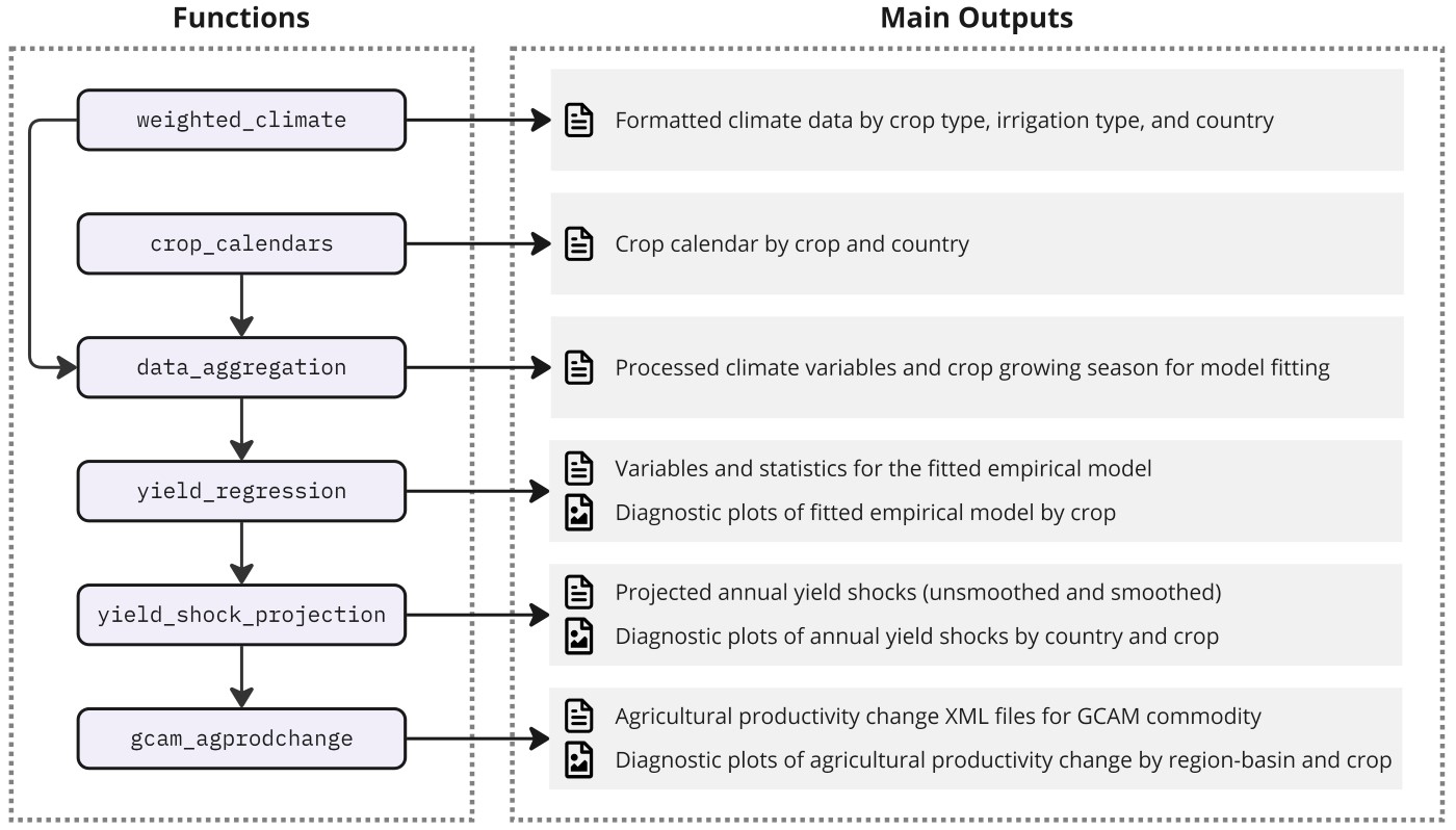
Figure 1: The gaia workflow showing the functions and the corresponding outputs of modeling crop yield shocks to climate variations using empirical econometric model.
Example Climate Data
gaia requires global climate data from the
Inter-Sectoral Impact Model Intercomparison Project (ISIMIP) or data formatted according
to ISIMIP
simulation protocols. Additionally, gaia supports
climate data in both daily and monthly time step. Due to the large size
of global climate data, we provide two types of example datasets
tailored to different user needs.
Example Data 1: This pre-processed climate dataset allows users to quickly run
gaiawithout the need to process raw climate NetCDF data. It is an output from thegaia::weighted_climatefunction, which converts raw climate NetCDF data into cropland-weighted climate data by country. This dataset includes both historical and future pre-processed cropland-weighted precipitation and temperature by country. If you want to quickly testgaiaand view the outputs, this is the easiest way to get started.Example Data 2: This climate dataset is designed for users who want to process raw climate NetCDF data using the
gaia::weighted_climatefunction. It includes global monthly precipitation and temperature NetCDF files at a 0.5-degree resolution, covering the period from 2015 to 2030. The example climate data is derived from the CanESM5 global climate model (GCM) under the Shared Socioeconomic Pathway-Representative Concentration Pathway (SSP-RCP) 2-4.5 scenario (O’Neil et al., 2016), also referred to as SSP245, as part of the CMIP6 projections (Swart et al., 2019). This climate projection has been bias-adjusted and statistically downscaled using the ISIMIP3BASD v2.5.0 approach (Lange, 2021; Lange, 2019). Processing this data may take some time. Please note that the selection of GCMs and SSP-RCP scenarios is not part ofgaiaframework. This dataset is provided solely for demonstration purpose. Users should choose climate projections that align with their research objectives. If you intend to use your own climate datasets, this example will serve as a helpful reference for setting up your workflow.
NOTE!
ISIMIP provides a range of bias-adjusted and statistically downscaled climate forcing data at a 0.5-degree resolution. Bias adjustment is the process of statistically modifying climate model outputs to better align with observed climate data, thereby reducing systematic errors or biases. To ensure consistency, simulated climate data should be bias-adjusted using the same historical climate observations that were used to fit the empirical model. For example, ISIMIP’s current CMIP6 climate outputs are bias-adjusted against the W5E5 v2.0 climate dataset using the ISIMIP3BASD v2.5.0 approach.
If you plan to use other climate observations or simulations that are not directly from ISIMIP, please ensure that you:
- Bias-adjust and statistically downscale your data to 0.5-degree resolution. You can follow ISIMIP’s official ISIMIP3BASD v2.5.0 approach (Lange, 2021; Lange, 2019), or use the basd software developed by the Pacific Northwest National Laboratory.
- Format your data according to ISIMIP’s guidelines for preparing simulation files in terms of NetCDF headers, grid format, variables and dimensions, and the time axis. More tips can be found here.
Example Data 1: Quick Start Dataset
Download the example data 1 using the instructions below. This
dataset includes both historical climate observations (1951-2001) and
future climate projections (2015-2100), weighted by cropland areas and
formatted in a tabular structure (see Table 1), as
required by gaia. The historical climate is from Water
and Global Change (WATCH) forcing data (Weedon et al., 2011)
and the climate projection is derived from CanESM5
under SSP245 scenario (Swart et al., 2019).
The cropland-area-weighted, country-level climate data contains monthly
precipitation and temperature for 26 crop types, distinguishing between
irrigated and rainfed areas.
There are two options to download the data:
-
Option 1: Please use this download
url and set the
data_dirto the directory of the downloaded folder;
data_dir <- 'path/to/downloaded/folder'-
Option 2: Use
gaia::get_example_datafunction following the code chunk below.
# load gaia
library(gaia)

# Path to the output folder. Change it to your desired location
output_dir <- 'gaia_example/example_climate'

# Cropland-weighted historical and future climate data
data_dir <- gaia::get_example_data(
  download_url = 'https://zenodo.org/records/14888816/files/weighted_climate.zip?download=1',
  data_dir = output_dir
)
Then, set the paths to historical and future climate data folder.
# Path to the folder that holds cropland-area-weighted precipitation and temperature TXT files
# historical climate observation
climate_hist_dir <- file.path(data_dir, 'climate_hist')
# future projected climate
climate_impact_dir <- file.path(data_dir, 'canesm5')
NOTE!
The default example historical climate data provided in example data 1 is based
on WATCH climate observations (Weedon et al., (2011)),
which were used in Waldhoff et al.,
(2020) for empirical model fitting. If you do not intend to modify
any assumptions or historical climate forcing for empirical model
fitting, you can use the default regression model in gaia,
which is pre-fitted with WATCH historical climate data, by setting the
argument use_default_coeff = TRUE. After loading the
gaia package, type coef_default to view the
parameters of the default pre-fitted model. Alternatively, if you prefer
to use different historical climate data other than the one from example data 1, you can
use weighted_climate function to generate cropland-weighted
historical monthly precipitation and temperature following the weighted_climate instruction under Explore Outputs section.
Example Data 2: Raw Climate Data
Download the example data 2 using the instructions below. This
dataset includes future global monthly precipitation and temperature
from 2015 to 2030 at 0.5-degree resolution, projected by CanESM5 global
climate model under SSP245 scenario. To use a different climate model or
scenario, users can provide their own climate data in NetCDF format.
Note that gaia adheres to the ISIMIP climate data format as
its standard, so your NetCDF files should be formatted accordingly if
the data is not directly downloaded from ISIMIP. More details on ISIMIP
format can be found in Tips for Formatting Climate
Forcing NetCDF section.
There are two options to download the data:
-
Option 1: Please use this download
url and set the
data_dirto the directory of the downloaded folder;
data_dir <- 'path/to/downloaded/folder'-
Option 2: Use
gaia::get_example_datafunction following the code chunk below.
# load gaia
library(gaia)

# Path to the output folder. Change it to your desired location
output_dir <- 'gaia_example/example_climate'

# Future Climate Data
data_dir <- gaia::get_example_data(
  download_url = 'https://zenodo.org/records/14888816/files/gaia_example_climate.zip?download=1',
  data_dir = output_dir
)
Then, set the paths to each of the climate files.
# Path to the precipitation and temperature NetCDF files
# NOTE: Each variable can have more than one file
# projected climate data
pr_projection_file <- file.path(data_dir, 'pr_monthly_canesm5_w5e5_ssp245_2015_2030.nc')
tas_projection_file <- file.path(data_dir, 'tas_monthly_canesm5_w5e5_ssp245_2015_2030.nc')
If you have your own climate forcing data, please follow the guidance
below to format your data to be compatible with gaia.
Tips for Formatting Climate Forcing NetCDF (Click to Expand the Content)
Formatting Your Climate Forcing Data for gaia
gaia requires that the climate NetCDF files follow the
basic formatting rules, specifically in terms of variables and
dimensions, spatial resolution, and attributes instructed in ISIMIP
protocols. The followings are some of the general
formatting requirements from ISIMIP that are compatible with
gaia.
Variables and Dimensions
- Variable names for precipitation and temperature should be
prandtas, respectively. - Every dimension should have an associated coordinate variable. For
prandtas, they should include three dimensions (coordinate variables):time,lon, andlat. - Precision of output variable is float.
- Precision of lon, lat and time should be double.
- First dimension should always be time.
- Identifier of dimensions and variables are all lowercase without spaces.
- For internal name of dimensions (coordinate variables), standard_name, long_name, unit and axis follow the conventions in the table below – the long_name definitions are not critical for the dimensions, but will give us warnings during the format checks.
Spatial Grid Resolution
Global grid ranges 89.75 to -89.75° latitude, and ‐179.75 to 179.75° longitude, i.e. 0.5° grid spacing, 360 rows and 720 columns, or 259200 grid cells total (corresponding to the resolution of the climate input data).
- Please report the output data row-wise starting at 89.75 and -179.75, and ending at -89.75 and 179.75.
- Reporting intervals are 0.5 degrees_east for longitude, and -0.5 degrees_north for latitude.
- CDO gridtype should be lonlat (not generic). This requires the longitude and latitude variable and dimension to be named ‘lon’ and ‘lat’.
- Grid points you do not simulate should be filled with the missing_value and _FillValue marker (1.e+20f).
Attributes
- Each variable’s attribute should at least include the units.
prshould be in the unit of kg m-2 s-1, andtasshould be in the unit of K.
A Standar NetCDF header should look like this:
 dimensions:
   lon = 720 ;
   lat = 360 ;
   time = UNLIMITED ;
variables:
   double lon(lon) ;
       lon:standard_name = "longitude" ;
       lon:long_name = "Longitude" ;
       lon:units = "degrees_east" ;
       lon:axis = "X" ;

   double lat(lat) ;
       lat:standard_name = "latitude" ;
       lat:long_name = "Latitude" ;
       lat:units = "degrees_north" ;
       lat:axis = "Y" ;

   double time(time) ;
       time:standard_name = "time" ;
       lat:long_name = "Time" ;
       time:units = "days since 1661-01-01 00:00:00" ;
       time:calendar = "proleptic_gregorian" ;
       time:axis = "T" ;

   float tas(time, lat, lon) ;
       tas:_FillValue = 1.e+20f ;
       tas:missing_value = 1.e+20f ;
       tas:units = “K" ;
       tas:standard_name = "air_temperature" ;
       tas:long_name = “Near-Surface Air Temperature" ;

// global attributes:
       :contact = "Your Contact Info <email>";
       :institution = "Your Institution";
       :comment = "Your comments" ;
Run gaia!
Example 1
WARNING!
This example demonstrates the complete gaia model workflow,
including processing the raw climate NetCDF data. Due to the large size
of the climate dataset, this process may take up to an hour. For a
quicker demonstration, please refer to Example
2.
This example guides users through the complete gaia
workflow, from processing raw climate data to calculating yield shocks
in response to future climate variations. Please note that we provide
only the NetCDF files for future climate from example data 2. For
historical model fitting, we use the pre-processed historical climate
data from example data
1 to reduce computational demands, especially for users without
access to high-performance computing.
If users have their own historical climate data for model fitting,
they can easily integrate it by specifying the paths to their historical
precipitation and temperature NetCDF files using the
pr_hist_ncdf and tas_hist_ncdf arguments,
respectively. Be sure to set climate_hist_dir = NULL to
bypass the pre-processed historical dataset.
Users can run gaia using the single function
yield_impact with our example data, which streamlines the
entire workflow. For detailed explanations of each argument in
yield_impact, please refer to the reference
page.
Intermediate outputs will be generated and saved to the user-specified output folder.
# load gaia
library(gaia)

# Path to the output folder. Change it to your desired location
output_dir <- 'gaia_example/example_1_output'

# Run gaia
# The full run with raw future climate data can take up to an hour
gaia::yield_impact(
  pr_hist_ncdf = NULL,                    # path to historical precipitation NetCDF file (must follow ISIMIP format); only if you wish to use your own historical precipitation observation
  tas_hist_ncdf = NULL,                   # path to historical temperature NetCDF file (must follow ISIMIP format); only if you wish to use your own historical temperature observation
  pr_proj_ncdf = pr_projection_file,      # path to future projected precipitation NetCDF file (must follow ISIMIP format)
  tas_proj_ncdf = tas_projection_file,    # path to future projected temperature NetCDF file (must follow ISIMIP format)
  timestep = 'monthly',                   # specify the time step of the NetCDF data (monthly or daily)
  climate_hist_dir = climate_hist_dir,    # path to the folder that holds cropland weighted historical climate observations
  historical_periods = c(1960:2001),      # vector of historical years selected for fitting
  climate_model = 'canesm5',              # label of climate model name
  climate_scenario = 'ssp245',            # label of climate scenario name
  member = 'r1i1p1f1',                    # label of ensemble member name
  bias_adj = 'w5e5',                      # label of climate data for bias adjustment for the global climate model (GCM)
  cfe = 'no-cfe',                         # label of CO2 fertilization effect in the formula (default is no CFE)
  gcam_version = 'gcam7',                 # output is different depending on the GCAM version (gcam6 or gcam7)
  use_default_coeff = FALSE,              # set to TRUE when there is no historical climate data available
  base_year = 2015,                       # GCAM base year
  start_year = 2015,                      # start year of the projected climate data
  end_year = 2030,                        # end year of the projected climate data
  smooth_window = 20,                     # number of years as smoothing window
  co2_hist = NULL,                        # historical annual CO2 concentration. If NULL, will use default value
  co2_proj = NULL,                        # projected annual CO2 concentration. If NULL, will use default value
  crop_select = NULL,                     # set to NULL for the default crops
  diagnostics = TRUE,                     # set to TRUE to output diagnostic plots
  output_dir = output_dir                 # path to the output folder
)
NOTE!
The arguments climate_model, climate_scenario,
member, bias_adj, and cfe require
specific strings that provide climate model metadata in the output
files. These arguments do not impact the gaia model
simulation itself; they are only used to populate climate data metadata
in the outputs.
Example 2
This example only uses the example of weighted climate
data as described in example data 1, which has
been processed with cropland weights at the country level. This weighted
climate data was generated using gaia::weighted_climate.
This example serves as a guide to help users format their own data to
match the weighted climate data structure if their raw climate data
differs from the ISIMIP format. Running gaia directly with
weighted climate data requires only a few minutes.
# load gaia
library(gaia)

# Path to the output folder. Change it to your desired location
output_dir <- 'gaia_example/example_2_output'

# Run gaia
gaia::yield_impact(
  climate_hist_dir = climate_hist_dir,    # path to the folder that holds cropland weighted historical climate observations
  climate_impact_dir = climate_impact_dir,# path to the folder that holds cropland weighted projected climate
  timestep = 'monthly',                   # specify the time step of the NetCDF data (monthly or daily)
  climate_model = 'canesm5',              # label of climate model name
  climate_scenario = 'ssp245',            # label of climate scenario name
  member = 'r1i1p1f1',                    # label of ensemble member name
  bias_adj = 'w5e5',                      # label of climate data for bias adjustment
  cfe = 'no-cfe',                         # label of CO2 fertilization effect in the formula (default is no CFE)
  gcam_version = 'gcam7',                 # output is different depending on the GCAM version (gcam6 or gcam7)
  use_default_coeff = FALSE,              # set to TRUE when there is no historical climate data available
  base_year = 2015,                       # GCAM base year
  start_year = 2015,                      # start year of the projected climate data
  end_year = 2100,                        # end year of the projected climate data
  smooth_window = 20,                     # number of years as smoothing window
  co2_hist = NULL,                        # historical annual CO2 concentration. If NULL, will use default value
  co2_proj = NULL,                        # projected annual CO2 concentration. If NULL, will use default value
  crop_select = NULL,                     # set to NULL for the default crops
  diagnostics = TRUE,                     # set to TRUE to output diagnostic plots
  output_dir = output_dir                 # path to the output folder
)
As stated in the previous note, if users plan to
use the WATCH forcing data from our example data 1 for
empirical model fitting, gaia has already stored the
corresponding fitted coefficients. To use these pre-fitted regression
coefficients, simply set use_default_coeff = TRUE and
climate_hist_dir = NULL in the example above. This simply
save some time to rerun the model regression. However, the pre-fitted
coefficients are only available for limited selection of 17 crops,
including barley, cassava, cotton, groundnuts, maize, millet, pulses,
rape_seed, rice, root_tuber, rye, sorghum, soybean, sugarbeet,
sugarcane, sunflower, and wheat.
If you want to include new crops beyond these 17 crops, you will need to provide the data on their planting and harvesting times to update the crop calendars (see instructions in crop_calendars). Then, you need to provide historical climate forcing data following either Example 1 or Example 2 to conduct the empirical fitting for those new crops.
Both Example 1 or Example 2 will generate intermediate and final outputs. Explore the results in your output folder. For a detailed explanation of the outputs, checkout Explore Outputs section!
Explore Outputs
Example 1 and Example
2 demonstrate how to use the wrapper function
yield_impact to streamline the entire workflows shown in Figure 1.
In this Section, we provide additional details on using each function described in the Workflow Overview section with the example data and explain the associated outputs and diagnostic plots if any. This section can help you better understand the workflow and the structure of the outputs, and allow you to make changes to certain steps (e.g., crop calendars) if needed.
If you have run Example 1 or Example 2 successfully, you should have all the
outputs available. However, you may choose to run the code snippet
within each subsection to regenerate these outputs if you prefer. Please
note that running the following code snippets will overwrite the
existing outputs in the corresponding output_dir.
weighted_climate
weighted_climate function calculates the
cropland-weighted monthly precipitation and temperature for the
projected climate. This function can be used if you wish to calculate
cropland-weighted monthly precipitation and temperature using different
climate forcing data. Please ensure that the climate NetCDF files
follows the ISIMIP
simulation protocols. Our example data 1 includes
the standard ISIMIP-style climate data for users to check the data
structure and format.
The example below uses the monthly precipitation (mm) and temperature
(degree C) projections from 2015 to 2030 To run this climate data
processing, please provide the file paths for the precipitation and
temperature NetCDF files using the pr_ncdf and
tas_ncdf arguments, respectively, and adjust the other
arguments accordingly to match the specifics of your climate data.
Please note that this step may take up to 10 minutes to complete.
library(gaia)

# Path to the output folder where you wish to save the outputs. Change it accordingly
output_dir <- 'gaia_example/example_1_output'

# calculate weigted climate
weighted_climate(pr_ncdf = pr_projection_file ,
                 tas_ncdf = tas_projection_file ,
                 timestep = 'monthly',
                 climate_model = 'canesm5',
                 climate_scenario = 'ssp245',
                 time_periods = seq(2015, 2030, 1),
                 output_dir = output_dir,
                 name_append = NULL)
The example above will create a folder based on the specified
climate_model argument (e.g.,
output_dir/weighted_climate/canesm5). Inside this folder,
you will find files containing precipitation and temperature data
weighted by the irrigated and rainfed cropland areas for 26 MIRCA2000
crops at the country level. The file structure is organized in columns
as follows: [year, month, 1, 2, 3, ..., 265], where the
numbers correspond to country IDs. To view the country names associated
with these IDs, simply type gaia::country_id in the R
console after loading the gaia package.
Outputs of the function: The function has no return
values. It writes the following output files to the
output_dir/weighted_climate folder:
[climate-model]_[climate-scenario]_month_precip_country_irc_[crop-number]_[start-year]_[end-year].csv: This file is the irrigated cropland-area weighted precipitation for certain climate model, scenario, and crop.[climate-model]_[climate-scenario]_month_precip_country_rfd_[crop-number]_[start-year]_[end-year].csv: This file is the rainfed cropland-area weighted precipitation for certain climate model, scenario, and crop.[climate-model]_[climate-scenario]_month_tmean_country_irc_[crop-number]_[start-year]_[end-year].csv: This file is the irrigated cropland-area weighted temperature for certain climate model, scenario, and crop.[climate-model]_[climate-scenario]_month_tmean_country_rfd_[crop-number]_[start-year]_[end-year].csv: This file is the rainfed cropland-area weighted temperature for certain climate model, scenario, and crop.
Below is an example of the structure for the weighted precipitation data for rainfed soybean.
| year | month | 1 | 2 | 3 | 4 | 5 | 6 | 7 | 8 | 9 | 10 | 11 | 12 | 13 | 14 | 15 | 16 | 17 | 18 | 19 | 20 | 21 | 22 | 23 | 24 | 25 | 26 | 27 | 28 | 29 | 30 | 31 | 32 | 33 | 34 | 35 | 36 | 37 | 38 | 39 | 40 | 41 | 42 | 43 | 44 | 45 | 46 | 47 | 48 | 49 | 50 | 51 | 52 | 53 | 54 | 55 | 56 | 57 | 58 | 59 | 60 | 61 | 62 | 63 | 64 | 65 | 66 | 67 | 68 | 69 | 70 | 71 | 72 | 73 | 74 | 75 | 76 | 77 | 78 | 79 | 80 | 81 | 82 | 83 | 84 | 85 | 86 | 87 | 88 | 89 | 90 | 91 | 92 | 93 | 94 | 95 | 96 | 97 | 98 | 99 | 100 | 101 | 102 | 103 | 104 | 105 | 106 | 107 | 108 | 109 | 110 | 111 | 112 | 113 | 114 | 115 | 116 | 117 | 118 | 119 | 120 | 121 | 122 | 123 | 124 | 125 | 126 | 127 | 128 | 129 | 130 | 131 | 132 | 133 | 134 | 135 | 136 | 137 | 138 | 139 | 140 | 141 | 142 | 143 | 144 | 145 | 146 | 147 | 148 | 149 | 150 | 151 | 152 | 153 | 154 | 155 | 156 | 157 | 158 | 159 | 160 | 161 | 162 | 163 | 164 | 165 | 166 | 167 | 168 | 169 | 170 | 171 | 172 | 173 | 174 | 175 | 176 | 177 | 178 | 179 | 180 | 181 | 182 | 183 | 184 | 185 | 186 | 187 | 188 | 189 | 190 | 191 | 192 | 193 | 194 | 195 | 196 | 197 | 198 | 199 | 200 | 201 | 202 | 203 | 204 | 205 | 206 | 207 | 208 | 209 | 210 | 211 | 212 | 213 | 214 | 215 | 216 | 217 | 218 | 219 | 220 | 221 | 222 | 223 | 224 | 225 | 226 | 227 | 228 | 229 | 230 | 231 | 232 | 233 | 234 | 235 | 236 | 237 | 238 | 239 | 240 | 241 | 242 | 243 | 244 | 245 | 246 | 247 | 248 | 249 | 250 | 251 | 252 | 253 | 254 | 255 | 256 | 257 | 258 | 259 | 260 | 261 | 262 | 263 | 264 | 265 |
|---|---|---|---|---|---|---|---|---|---|---|---|---|---|---|---|---|---|---|---|---|---|---|---|---|---|---|---|---|---|---|---|---|---|---|---|---|---|---|---|---|---|---|---|---|---|---|---|---|---|---|---|---|---|---|---|---|---|---|---|---|---|---|---|---|---|---|---|---|---|---|---|---|---|---|---|---|---|---|---|---|---|---|---|---|---|---|---|---|---|---|---|---|---|---|---|---|---|---|---|---|---|---|---|---|---|---|---|---|---|---|---|---|---|---|---|---|---|---|---|---|---|---|---|---|---|---|---|---|---|---|---|---|---|---|---|---|---|---|---|---|---|---|---|---|---|---|---|---|---|---|---|---|---|---|---|---|---|---|---|---|---|---|---|---|---|---|---|---|---|---|---|---|---|---|---|---|---|---|---|---|---|---|---|---|---|---|---|---|---|---|---|---|---|---|---|---|---|---|---|---|---|---|---|---|---|---|---|---|---|---|---|---|---|---|---|---|---|---|---|---|---|---|---|---|---|---|---|---|---|---|---|---|---|---|---|---|---|---|---|---|---|---|---|---|---|---|---|---|---|---|---|---|---|---|---|---|---|---|---|---|---|---|---|---|---|---|
| 2015 | 1 | -9999 | 4.03 | 53.86 | 69.98 | -9999 | 57.62 | 138.56 | -9999 | -9999 | -9999 | 59.05 | 18.86 | 1.70 | -9999 | 169.60 | 66.10 | 15.35 | -9999 | -9999 | -9999 | -9999 | 1.20 | -9999 | 40.87 | -9999 | 90.56 | 4.55 | -9999 | 1.02 | 223.33 | -9999 | 75.63 | 164.45 | -9999 | 194.95 | -9999 | -9999 | 51.34 | 0.49 | 0.81 | 55.25 | 3.27 | 1.49 | 94.46 | -9999 | -9999 | 4.01 | 0.32 | 3.71 | 6.32 | -9999 | -9999 | -9999 | 41.04 | -9999 | 47.70 | 110.07 | -9999 | -9999 | 75.42 | 73.39 | -9999 | -9999 | -9999 | 57.43 | 20.93 | 84.39 | 0.78 | -9999 | -9999 | 58.73 | 4.37 | 72.18 | 101.86 | 0.85 | 41.68 | 4.11 | -9999 | -9999 | -9999 | -9999 | -9999 | 28.02 | 92.94 | -9999 | -9999 | -9999 | 147.86 | -9999 | -9999 | 40.36 | 61.93 | 20.93 | -9999 | -9999 | 93.14 | -9999 | -9999 | -9999 | -9999 | 51.93 | -9999 | 3.41 | -9999 | 41.33 | -9999 | -9999 | 134.27 | 11.70 | -9999 | 68.14 | -9999 | 15.58 | 319.27 | 22.22 | 51.74 | -9999 | -9999 | 18.41 | 47.33 | -9999 | 96.38 | -9999 | -9999 | -9999 | 26.11 | -9999 | 33.48 | 14.74 | -9999 | -9999 | -9999 | 11.17 | 5.32 | 28.40 | 72.58 | 47.88 | 20.44 | -9999 | -9999 | 35.98 | -9999 | 5.20 | 36.93 | 284.14 | 161.40 | 27.04 | -9999 | 0.69 | -9999 | -9999 | -9999 | -9999 | -9999 | -9999 | 9.03 | -9999 | 23.32 | -9999 | 2.49 | -9999 | -9999 | 61.35 | 189.14 | 1.15 | -9999 | -9999 | 21.23 | -9999 | -9999 | -9999 | 79.40 | 0.09 | 1.48 | -9999 | -9999 | 6.52 | -9999 | -9999 | -9999 | 10.04 | -9999 | -9999 | -9999 | 44.26 | -9999 | 156.52 | 67.94 | 393.70 | -9999 | 38.45 | -9999 | -9999 | -9999 | -9999 | -9999 | 36.00 | 50.95 | -9999 | -9999 | -9999 | -9999 | -9999 | -9999 | -9999 | -9999 | -9999 | -9999 | -9999 | -9999 | -9999 | -9999 | -9999 | -9999 | -9999 | 51.12 | 117.86 | -9999 | 0.04 | 91.64 | -9999 | 34.83 | -9999 | -9999 | 30.59 | 3.91 | 244.94 | -9999 | -9999 | -9999 | 91.36 | 47.77 | 10.27 | 16.34 | 98.66 | 4.72 | 216.98 | -9999 | -9999 | -9999 | 24.50 | -9999 | -9999 | 57.03 | -9999 | -9999 | -9999 | 26.57 | 35.89 | -9999 | -9999 | 40.45 | 36.84 | -9999 | -9999 | 6.19 | 9.88 | -9999 | -9999 | -9999 | -9999 | -9999 | 182.50 | 159.87 | -9999 |
| 2015 | 2 | -9999 | 4.20 | 36.39 | 65.82 | -9999 | 89.91 | 161.89 | -9999 | -9999 | -9999 | 86.15 | 15.77 | 14.84 | -9999 | 58.85 | 72.13 | 15.67 | -9999 | -9999 | -9999 | -9999 | 0.17 | -9999 | 43.57 | -9999 | 150.81 | 4.72 | -9999 | 6.33 | 110.87 | -9999 | 73.55 | 44.94 | -9999 | 153.15 | -9999 | -9999 | 18.64 | 1.43 | 3.91 | 93.70 | 2.29 | 12.40 | 90.94 | -9999 | -9999 | 52.08 | 0.31 | 3.08 | 23.28 | -9999 | -9999 | -9999 | 48.96 | -9999 | 117.52 | 174.88 | -9999 | -9999 | 32.08 | 91.36 | -9999 | -9999 | -9999 | 52.39 | 52.70 | 82.44 | 10.85 | -9999 | -9999 | 79.17 | 4.39 | 78.45 | 238.82 | 4.32 | 73.35 | 29.84 | -9999 | -9999 | -9999 | -9999 | -9999 | 45.37 | 134.09 | -9999 | -9999 | -9999 | 308.04 | -9999 | -9999 | 13.18 | 48.76 | 40.96 | -9999 | -9999 | 15.89 | -9999 | -9999 | -9999 | -9999 | 52.03 | -9999 | 12.09 | -9999 | 100.10 | -9999 | -9999 | 214.62 | 67.03 | -9999 | 72.50 | -9999 | 5.40 | 309.64 | 7.48 | 19.63 | -9999 | -9999 | 7.82 | 106.90 | -9999 | 88.29 | -9999 | -9999 | -9999 | 10.24 | -9999 | 19.53 | 76.39 | -9999 | -9999 | -9999 | 13.10 | 4.33 | 51.62 | 29.70 | 66.05 | 33.60 | -9999 | -9999 | 46.48 | -9999 | 30.86 | 20.76 | 264.13 | 130.83 | 45.23 | -9999 | 0.27 | -9999 | -9999 | -9999 | -9999 | -9999 | -9999 | 15.71 | -9999 | 18.65 | -9999 | 7.00 | -9999 | -9999 | 144.19 | 67.72 | 11.68 | -9999 | -9999 | 42.90 | -9999 | -9999 | -9999 | 75.10 | 0.12 | 8.06 | -9999 | -9999 | 29.69 | -9999 | -9999 | -9999 | 62.13 | -9999 | -9999 | -9999 | 28.13 | -9999 | 120.08 | 100.14 | 265.95 | -9999 | 37.48 | -9999 | -9999 | -9999 | -9999 | -9999 | 27.08 | 115.64 | -9999 | -9999 | -9999 | -9999 | -9999 | -9999 | -9999 | -9999 | -9999 | -9999 | -9999 | -9999 | -9999 | -9999 | -9999 | -9999 | -9999 | 39.72 | 158.79 | -9999 | 6.61 | 52.38 | -9999 | 78.77 | -9999 | -9999 | 18.70 | 13.77 | 320.54 | -9999 | -9999 | -9999 | 130.48 | 20.21 | 73.92 | 20.14 | 156.96 | 1.35 | 103.35 | -9999 | -9999 | -9999 | 32.84 | -9999 | -9999 | 23.10 | -9999 | -9999 | -9999 | 64.13 | 25.47 | -9999 | -9999 | 65.72 | 68.58 | -9999 | -9999 | 14.66 | 12.15 | -9999 | -9999 | -9999 | -9999 | -9999 | 140.59 | 36.12 | -9999 |
| 2015 | 3 | -9999 | 7.97 | 54.74 | 39.23 | -9999 | 16.70 | 212.43 | -9999 | -9999 | -9999 | 54.12 | 14.97 | 1.19 | -9999 | 48.51 | 31.36 | 8.97 | -9999 | -9999 | -9999 | -9999 | 51.33 | -9999 | 28.96 | -9999 | 15.97 | 16.47 | -9999 | 72.28 | 130.70 | -9999 | 65.13 | 45.21 | -9999 | 138.26 | -9999 | -9999 | 88.01 | 0.39 | 31.48 | 54.27 | 18.96 | 98.74 | 83.20 | -9999 | -9999 | 161.43 | 0.35 | 1.45 | 25.46 | -9999 | -9999 | -9999 | 78.17 | -9999 | 225.21 | 191.02 | -9999 | -9999 | 34.07 | 49.60 | -9999 | -9999 | -9999 | 32.57 | 54.49 | 34.37 | 3.40 | -9999 | -9999 | 87.02 | 2.55 | 16.11 | 277.63 | 1.42 | 24.77 | 13.13 | -9999 | -9999 | -9999 | -9999 | -9999 | 19.15 | 29.83 | -9999 | -9999 | -9999 | 544.38 | -9999 | -9999 | 52.19 | 35.45 | 37.90 | -9999 | -9999 | 57.30 | -9999 | -9999 | -9999 | -9999 | 15.00 | -9999 | 57.94 | -9999 | 25.82 | -9999 | -9999 | 25.46 | 47.62 | -9999 | 61.36 | -9999 | 1.58 | 256.66 | 15.37 | 23.64 | -9999 | -9999 | 5.51 | 33.55 | -9999 | 92.29 | -9999 | -9999 | -9999 | 5.80 | -9999 | 41.97 | 74.57 | -9999 | -9999 | -9999 | 33.20 | 40.21 | 17.33 | 23.56 | 35.58 | 88.31 | -9999 | -9999 | 20.36 | -9999 | 20.55 | 38.96 | 176.13 | 141.25 | 123.62 | -9999 | 0.24 | -9999 | -9999 | -9999 | -9999 | -9999 | -9999 | 3.36 | -9999 | 41.89 | -9999 | 2.89 | -9999 | -9999 | 20.43 | 88.88 | 4.59 | -9999 | -9999 | 8.71 | -9999 | -9999 | -9999 | 28.71 | 0.50 | 35.80 | -9999 | -9999 | 34.61 | -9999 | -9999 | -9999 | 8.55 | -9999 | -9999 | -9999 | 34.39 | -9999 | 126.60 | 84.93 | 192.78 | -9999 | 22.62 | -9999 | -9999 | -9999 | -9999 | -9999 | 44.38 | 68.91 | -9999 | -9999 | -9999 | -9999 | -9999 | -9999 | -9999 | -9999 | -9999 | -9999 | -9999 | -9999 | -9999 | -9999 | -9999 | -9999 | -9999 | 22.07 | 63.51 | -9999 | 5.56 | 40.41 | -9999 | 60.19 | -9999 | -9999 | 202.11 | 81.39 | 114.82 | -9999 | -9999 | -9999 | 68.29 | 18.24 | 59.03 | 40.70 | 64.77 | 22.09 | 138.37 | -9999 | -9999 | -9999 | 16.22 | -9999 | -9999 | 31.30 | -9999 | -9999 | -9999 | 123.70 | 49.80 | -9999 | -9999 | 57.23 | 73.46 | -9999 | -9999 | 7.18 | 48.95 | -9999 | -9999 | -9999 | -9999 | -9999 | 136.98 | 60.31 | -9999 |
| 2015 | 4 | -9999 | 2.63 | 26.55 | 26.88 | -9999 | 23.01 | 127.63 | -9999 | -9999 | -9999 | 50.17 | 29.37 | 3.43 | -9999 | 52.47 | 46.87 | 14.89 | -9999 | -9999 | -9999 | -9999 | 169.96 | -9999 | 59.04 | -9999 | 43.52 | 51.63 | -9999 | 191.59 | 71.12 | -9999 | 55.76 | 14.98 | -9999 | 66.22 | -9999 | -9999 | 26.85 | 15.01 | 63.43 | 87.82 | 77.54 | 65.91 | 100.36 | -9999 | -9999 | 315.15 | 0.82 | 1.42 | 66.52 | -9999 | -9999 | -9999 | 203.84 | -9999 | 199.77 | 115.82 | -9999 | -9999 | 37.72 | 55.99 | -9999 | -9999 | -9999 | 32.39 | 90.86 | 68.94 | 8.86 | -9999 | -9999 | 160.76 | 0.04 | 51.96 | 381.37 | 14.87 | 26.00 | 61.93 | -9999 | -9999 | -9999 | -9999 | -9999 | 15.75 | 46.43 | -9999 | -9999 | -9999 | 448.85 | -9999 | -9999 | 35.35 | 34.48 | 49.20 | -9999 | -9999 | 8.21 | -9999 | -9999 | -9999 | -9999 | 49.47 | -9999 | 144.31 | -9999 | 34.04 | -9999 | -9999 | 30.61 | 252.45 | -9999 | 102.21 | -9999 | 1.02 | 231.08 | 5.97 | 3.62 | -9999 | -9999 | 4.39 | 38.12 | -9999 | 130.18 | -9999 | -9999 | -9999 | 4.39 | -9999 | 22.65 | 191.58 | -9999 | -9999 | -9999 | 12.04 | 101.60 | 24.40 | 14.13 | 23.42 | 195.93 | -9999 | -9999 | 17.87 | -9999 | 106.78 | 16.50 | 178.83 | 27.81 | 69.59 | -9999 | 10.27 | -9999 | -9999 | -9999 | -9999 | -9999 | -9999 | 1.34 | -9999 | 14.55 | -9999 | 15.67 | -9999 | -9999 | 5.07 | 36.98 | 11.34 | -9999 | -9999 | 16.18 | -9999 | -9999 | -9999 | 18.63 | 1.32 | 40.28 | -9999 | -9999 | 36.92 | -9999 | -9999 | -9999 | 13.18 | -9999 | -9999 | -9999 | 84.18 | -9999 | 108.34 | 65.92 | 115.00 | -9999 | 46.56 | -9999 | -9999 | -9999 | -9999 | -9999 | 36.12 | 107.80 | -9999 | -9999 | -9999 | -9999 | -9999 | -9999 | -9999 | -9999 | -9999 | -9999 | -9999 | -9999 | -9999 | -9999 | -9999 | -9999 | -9999 | 74.99 | 91.42 | -9999 | 19.34 | 27.23 | -9999 | 92.19 | -9999 | -9999 | 79.45 | 95.30 | 120.02 | -9999 | -9999 | -9999 | 66.02 | 14.62 | 249.47 | 12.77 | 74.19 | 103.67 | 174.35 | -9999 | -9999 | -9999 | 21.85 | -9999 | -9999 | 46.14 | -9999 | -9999 | -9999 | 250.33 | 35.77 | -9999 | -9999 | 69.07 | 84.54 | -9999 | -9999 | 26.22 | 81.51 | -9999 | -9999 | -9999 | -9999 | -9999 | 10.24 | 16.20 | -9999 |
| 2015 | 5 | -9999 | 0.49 | 58.51 | 1.98 | -9999 | 17.21 | 10.84 | -9999 | -9999 | -9999 | 69.00 | 43.85 | 0.63 | -9999 | 134.07 | 73.22 | 35.13 | -9999 | -9999 | -9999 | -9999 | 352.93 | -9999 | 33.65 | -9999 | 40.04 | 283.29 | -9999 | 493.23 | 22.07 | -9999 | 79.62 | 7.28 | -9999 | 34.24 | -9999 | -9999 | 54.18 | 100.75 | 145.36 | 22.32 | 108.05 | 148.98 | 116.81 | -9999 | -9999 | 121.60 | 21.77 | 0.64 | 63.15 | -9999 | -9999 | -9999 | 239.41 | -9999 | 156.80 | 16.91 | -9999 | -9999 | 177.28 | 84.92 | -9999 | -9999 | -9999 | 51.68 | 228.77 | 67.92 | 8.82 | -9999 | -9999 | 110.27 | 1.12 | 72.65 | 322.82 | 7.26 | 54.37 | 29.37 | -9999 | -9999 | -9999 | -9999 | -9999 | 24.73 | 56.26 | -9999 | -9999 | -9999 | 219.43 | -9999 | -9999 | 36.98 | 81.92 | 304.63 | -9999 | -9999 | 39.69 | -9999 | -9999 | -9999 | -9999 | 56.23 | -9999 | 142.49 | -9999 | 86.60 | -9999 | -9999 | 66.85 | 153.45 | -9999 | 95.32 | -9999 | 11.98 | 103.80 | 11.77 | 14.78 | -9999 | -9999 | 4.67 | 98.61 | -9999 | 138.66 | -9999 | -9999 | -9999 | 2.52 | -9999 | 39.24 | 97.09 | -9999 | -9999 | -9999 | 2.34 | 145.29 | 43.36 | 12.85 | 5.38 | 204.93 | -9999 | -9999 | 29.60 | -9999 | 96.97 | 49.53 | 50.06 | 4.48 | 169.39 | -9999 | 64.34 | -9999 | -9999 | -9999 | -9999 | -9999 | -9999 | 10.70 | -9999 | 21.51 | -9999 | 23.38 | -9999 | -9999 | 9.23 | 8.59 | 0.33 | -9999 | -9999 | 89.76 | -9999 | -9999 | -9999 | 109.36 | 36.62 | 219.58 | -9999 | -9999 | 37.54 | -9999 | -9999 | -9999 | 1.40 | -9999 | -9999 | -9999 | 234.78 | -9999 | 98.74 | 41.12 | 134.41 | -9999 | 31.74 | -9999 | -9999 | -9999 | -9999 | -9999 | 47.85 | 34.28 | -9999 | -9999 | -9999 | -9999 | -9999 | -9999 | -9999 | -9999 | -9999 | -9999 | -9999 | -9999 | -9999 | -9999 | -9999 | -9999 | -9999 | 47.04 | 145.54 | -9999 | 10.46 | 10.47 | -9999 | 78.28 | -9999 | -9999 | 171.13 | 84.03 | 169.03 | -9999 | -9999 | -9999 | 186.44 | 14.71 | 137.64 | 3.40 | 12.52 | 193.16 | 34.83 | -9999 | -9999 | -9999 | 66.41 | -9999 | -9999 | 38.37 | -9999 | -9999 | -9999 | 121.28 | 22.77 | -9999 | -9999 | 120.41 | 32.17 | -9999 | -9999 | 87.33 | 94.79 | -9999 | -9999 | -9999 | -9999 | -9999 | 1.19 | 4.42 | -9999 |
| 2015 | 6 | -9999 | 8.85 | 45.99 | 19.61 | -9999 | 8.10 | 1.30 | -9999 | -9999 | -9999 | 22.89 | 18.77 | 7.06 | -9999 | 62.68 | 85.73 | 8.86 | -9999 | -9999 | -9999 | -9999 | 503.91 | -9999 | 85.89 | -9999 | 180.09 | 114.58 | -9999 | 1036.57 | 19.10 | -9999 | 64.53 | 3.03 | -9999 | 38.35 | -9999 | -9999 | 54.44 | 42.05 | 121.39 | 4.35 | 161.40 | 117.74 | 121.67 | -9999 | -9999 | 87.32 | 41.38 | -9999.00 | 102.89 | -9999 | -9999 | -9999 | 231.66 | -9999 | 5.85 | 3.74 | -9999 | -9999 | 401.24 | 59.72 | -9999 | -9999 | -9999 | 88.63 | 147.90 | 61.72 | 14.70 | -9999 | -9999 | 110.36 | 0.05 | 171.50 | 51.78 | 52.67 | 69.19 | 57.75 | -9999 | -9999 | -9999 | -9999 | -9999 | 34.69 | 22.36 | -9999 | -9999 | -9999 | 50.45 | -9999 | -9999 | 32.43 | 49.23 | 90.97 | -9999 | -9999 | 14.67 | -9999 | -9999 | -9999 | -9999 | 128.71 | -9999 | 253.50 | -9999 | 130.95 | -9999 | -9999 | 248.13 | 360.98 | -9999 | 98.26 | -9999 | 121.03 | 102.76 | 0.46 | 0.42 | -9999 | -9999 | 0.21 | 43.43 | -9999 | 133.08 | -9999 | -9999 | -9999 | 0.13 | -9999 | 29.05 | 34.97 | -9999 | -9999 | -9999 | 7.90 | 143.40 | 52.36 | 1.09 | 2.55 | 345.38 | -9999 | -9999 | 52.16 | -9999 | 147.68 | 31.11 | 30.01 | 2.65 | 149.67 | -9999 | 35.62 | -9999 | -9999 | -9999 | -9999 | -9999 | -9999 | 16.18 | -9999 | 74.25 | -9999 | 53.76 | -9999 | -9999 | 18.65 | 3.23 | 10.49 | -9999 | -9999 | 171.14 | -9999 | -9999 | -9999 | 348.32 | 26.10 | 109.30 | -9999 | -9999 | 21.42 | -9999 | -9999 | -9999 | 61.94 | -9999 | -9999 | -9999 | 347.26 | -9999 | 81.88 | 45.13 | 177.46 | -9999 | 83.20 | -9999 | -9999 | -9999 | -9999 | -9999 | 59.88 | 6.45 | -9999 | -9999 | -9999 | -9999 | -9999 | -9999 | -9999 | -9999 | -9999 | -9999 | -9999 | -9999 | -9999 | -9999 | -9999 | -9999 | -9999 | 83.30 | 87.26 | -9999 | 10.12 | 11.75 | -9999 | 41.19 | -9999 | -9999 | 105.05 | 30.31 | 278.96 | -9999 | -9999 | -9999 | 76.66 | 1.45 | 241.29 | 5.61 | 7.65 | 138.01 | 57.36 | -9999 | -9999 | -9999 | 150.30 | -9999 | -9999 | 5.81 | -9999 | -9999 | -9999 | 45.86 | 90.97 | -9999 | -9999 | 92.79 | 61.27 | -9999 | -9999 | 126.81 | 121.68 | -9999 | -9999 | -9999 | -9999 | -9999 | 0.26 | 0.66 | -9999 |
| 2015 | 7 | -9999 | 9.69 | 2.97 | 8.08 | -9999 | 12.09 | 0.20 | -9999 | -9999 | -9999 | 31.95 | 18.62 | 9.77 | -9999 | 22.70 | 49.87 | 13.41 | -9999 | -9999 | -9999 | -9999 | 308.84 | -9999 | 111.83 | -9999 | 191.70 | 122.70 | -9999 | 318.96 | 12.60 | -9999 | 16.15 | 0.27 | -9999 | 14.92 | -9999 | -9999 | 49.87 | 76.88 | 200.72 | 5.14 | 138.15 | 185.49 | 57.76 | -9999 | -9999 | 153.41 | 91.20 | 0.60 | 160.79 | -9999 | -9999 | -9999 | 225.13 | -9999 | 5.92 | 4.59 | -9999 | -9999 | 254.23 | 30.27 | -9999 | -9999 | -9999 | 62.47 | 170.51 | 130.49 | 36.08 | -9999 | -9999 | 66.20 | 0.21 | 182.16 | 33.95 | 114.15 | 158.04 | 173.24 | -9999 | -9999 | -9999 | -9999 | -9999 | 47.68 | 35.03 | -9999 | -9999 | -9999 | 17.14 | -9999 | -9999 | 27.62 | 71.22 | 116.73 | -9999 | -9999 | 0.96 | -9999 | -9999 | -9999 | -9999 | 154.95 | -9999 | 276.61 | -9999 | 119.35 | -9999 | -9999 | 243.61 | 214.09 | -9999 | 39.47 | -9999 | 66.40 | 90.44 | 4.44 | 0.13 | -9999 | -9999 | 0.15 | 46.06 | -9999 | 155.75 | -9999 | -9999 | -9999 | 0.06 | -9999 | 58.43 | 105.91 | -9999 | -9999 | -9999 | 9.32 | 195.13 | 120.90 | 0.12 | 25.70 | 339.80 | -9999 | -9999 | 98.21 | -9999 | 113.18 | 1.42 | 48.27 | 4.00 | 174.31 | -9999 | 75.38 | -9999 | -9999 | -9999 | -9999 | -9999 | -9999 | 41.33 | -9999 | 60.59 | -9999 | 93.04 | -9999 | -9999 | 2.75 | 5.54 | 3.80 | -9999 | -9999 | 180.26 | -9999 | -9999 | -9999 | 391.33 | 94.09 | 166.32 | -9999 | -9999 | 377.29 | -9999 | -9999 | -9999 | 61.01 | -9999 | -9999 | -9999 | 227.77 | -9999 | 19.11 | 27.58 | 142.42 | -9999 | 62.23 | -9999 | -9999 | -9999 | -9999 | -9999 | 87.08 | 7.58 | -9999 | -9999 | -9999 | -9999 | -9999 | -9999 | -9999 | -9999 | -9999 | -9999 | -9999 | -9999 | -9999 | -9999 | -9999 | -9999 | -9999 | 37.91 | 83.26 | -9999 | 14.94 | 24.85 | -9999 | 300.88 | -9999 | -9999 | 61.24 | 130.12 | 238.12 | -9999 | -9999 | -9999 | 59.44 | 0.30 | 198.84 | 6.03 | 4.61 | 130.20 | 47.50 | -9999 | -9999 | -9999 | 127.95 | -9999 | -9999 | 2.63 | -9999 | -9999 | -9999 | 144.13 | 51.93 | -9999 | -9999 | 42.75 | 90.62 | -9999 | -9999 | 171.63 | 222.16 | -9999 | -9999 | -9999 | -9999 | -9999 | 0.50 | 0.43 | -9999 |
| 2015 | 8 | -9999 | 4.09 | 25.79 | 3.13 | -9999 | 18.30 | 47.74 | -9999 | -9999 | -9999 | 47.83 | 4.28 | 12.58 | -9999 | 32.84 | 84.92 | 4.43 | -9999 | -9999 | -9999 | -9999 | 269.85 | -9999 | 61.58 | -9999 | 240.92 | 150.45 | -9999 | 391.71 | 8.01 | -9999 | 60.37 | 2.60 | -9999 | 38.84 | -9999 | -9999 | 12.76 | 127.91 | 181.14 | 62.39 | 154.14 | 200.45 | 94.40 | -9999 | -9999 | 220.77 | 207.38 | -9999.00 | 88.00 | -9999 | -9999 | -9999 | 162.31 | -9999 | 51.30 | 66.62 | -9999 | -9999 | 299.46 | 91.78 | -9999 | -9999 | -9999 | 42.66 | 196.40 | 121.71 | 55.90 | -9999 | -9999 | 42.68 | 0.12 | 257.10 | 59.98 | 155.81 | 129.92 | 146.81 | -9999 | -9999 | -9999 | -9999 | -9999 | 79.98 | 29.68 | -9999 | -9999 | -9999 | 25.39 | -9999 | -9999 | 11.38 | 35.68 | 115.64 | -9999 | -9999 | 2.95 | -9999 | -9999 | -9999 | -9999 | 196.62 | -9999 | 402.79 | -9999 | 49.19 | -9999 | -9999 | 265.23 | 400.11 | -9999 | 88.49 | -9999 | 95.94 | 72.17 | 1.47 | 0.36 | -9999 | -9999 | 1.25 | 71.59 | -9999 | 106.57 | -9999 | -9999 | -9999 | 0.55 | -9999 | 29.19 | 205.72 | -9999 | -9999 | -9999 | 3.81 | 154.07 | 78.83 | 0.70 | 24.27 | 487.94 | -9999 | -9999 | 33.10 | -9999 | 265.90 | 15.99 | 25.48 | 0.90 | 183.75 | -9999 | 115.44 | -9999 | -9999 | -9999 | -9999 | -9999 | -9999 | 16.07 | -9999 | 25.65 | -9999 | 40.67 | -9999 | -9999 | 1.55 | 2.56 | 0.93 | -9999 | -9999 | 95.29 | -9999 | -9999 | -9999 | 368.71 | 136.16 | 194.12 | -9999 | -9999 | 136.98 | -9999 | -9999 | -9999 | 27.74 | -9999 | -9999 | -9999 | 257.62 | -9999 | 127.94 | 13.79 | 114.09 | -9999 | 36.73 | -9999 | -9999 | -9999 | -9999 | -9999 | 47.79 | 98.23 | -9999 | -9999 | -9999 | -9999 | -9999 | -9999 | -9999 | -9999 | -9999 | -9999 | -9999 | -9999 | -9999 | -9999 | -9999 | -9999 | -9999 | 61.90 | 188.29 | -9999 | 34.01 | 19.76 | -9999 | 219.06 | -9999 | -9999 | 131.52 | 195.68 | 124.75 | -9999 | -9999 | -9999 | 60.82 | 0.70 | 193.93 | 1.30 | 7.96 | 158.38 | 9.27 | -9999 | -9999 | -9999 | 63.12 | -9999 | -9999 | 5.27 | -9999 | -9999 | -9999 | 320.37 | 26.59 | -9999 | -9999 | 72.15 | 134.74 | -9999 | -9999 | 199.83 | 131.68 | -9999 | -9999 | -9999 | -9999 | -9999 | 0.18 | 0.32 | -9999 |
| 2015 | 9 | -9999 | 14.96 | 29.89 | 38.64 | -9999 | 18.42 | 51.19 | -9999 | -9999 | -9999 | 52.67 | 26.34 | 18.52 | -9999 | 55.47 | 37.81 | 27.77 | -9999 | -9999 | -9999 | -9999 | 380.73 | -9999 | 55.34 | -9999 | 206.89 | 111.78 | -9999 | 483.22 | 22.65 | -9999 | 34.68 | 0.30 | -9999 | 44.59 | -9999 | -9999 | 48.24 | 62.86 | 101.08 | 29.81 | 250.70 | 217.30 | 44.56 | -9999 | -9999 | 134.71 | 123.05 | 0.18 | 49.39 | -9999 | -9999 | -9999 | 191.26 | -9999 | 78.06 | 64.36 | -9999 | -9999 | 344.43 | 34.71 | -9999 | -9999 | -9999 | 40.72 | 261.46 | 63.26 | 22.02 | -9999 | -9999 | 44.77 | 0.11 | 198.14 | 287.66 | 56.34 | 35.57 | 75.11 | -9999 | -9999 | -9999 | -9999 | -9999 | 38.39 | 37.69 | -9999 | -9999 | -9999 | 145.39 | -9999 | -9999 | 17.11 | 50.38 | 139.89 | -9999 | -9999 | 35.90 | -9999 | -9999 | -9999 | -9999 | 155.60 | -9999 | 442.27 | -9999 | 39.96 | -9999 | -9999 | 334.11 | 118.49 | -9999 | 49.86 | -9999 | 452.91 | 85.62 | 6.66 | 1.13 | -9999 | -9999 | 0.25 | 31.89 | -9999 | 192.70 | -9999 | -9999 | -9999 | 0.05 | -9999 | 26.29 | 50.86 | -9999 | -9999 | -9999 | 1.66 | 126.05 | 21.02 | 0.27 | 26.08 | 494.01 | -9999 | -9999 | 28.94 | -9999 | 59.74 | 22.31 | 40.78 | 2.25 | 276.49 | -9999 | 50.56 | -9999 | -9999 | -9999 | -9999 | -9999 | -9999 | 24.63 | -9999 | 26.30 | -9999 | 16.70 | -9999 | -9999 | 20.52 | 2.26 | 1.58 | -9999 | -9999 | 812.71 | -9999 | -9999 | -9999 | 349.53 | 112.97 | 159.68 | -9999 | -9999 | 153.83 | -9999 | -9999 | -9999 | 111.42 | -9999 | -9999 | -9999 | 269.08 | -9999 | 105.57 | 35.54 | 173.39 | -9999 | 55.66 | -9999 | -9999 | -9999 | -9999 | -9999 | 54.44 | 44.04 | -9999 | -9999 | -9999 | -9999 | -9999 | -9999 | -9999 | -9999 | -9999 | -9999 | -9999 | -9999 | -9999 | -9999 | -9999 | -9999 | -9999 | 67.78 | 64.99 | -9999 | 17.87 | 12.61 | -9999 | 291.77 | -9999 | -9999 | 160.20 | 118.62 | 71.55 | -9999 | -9999 | -9999 | 64.54 | 1.22 | 128.60 | 1.78 | 4.77 | 177.59 | 42.10 | -9999 | -9999 | -9999 | 67.54 | -9999 | -9999 | 6.90 | -9999 | -9999 | -9999 | 95.06 | 38.02 | -9999 | -9999 | 58.87 | 116.68 | -9999 | -9999 | 150.89 | 114.61 | -9999 | -9999 | -9999 | -9999 | -9999 | 0.46 | 0.33 | -9999 |
| 2015 | 10 | -9999 | 0.15 | 24.62 | 65.74 | -9999 | 18.91 | 127.72 | -9999 | -9999 | -9999 | 54.73 | 32.07 | 43.50 | -9999 | 117.42 | 13.18 | 43.76 | -9999 | -9999 | -9999 | -9999 | 72.07 | -9999 | 37.02 | -9999 | 242.55 | 53.29 | -9999 | 54.03 | 51.46 | -9999 | 18.09 | 4.76 | -9999 | 127.78 | -9999 | -9999 | 26.50 | 18.62 | 82.85 | 95.02 | 269.41 | 119.51 | 63.94 | -9999 | -9999 | 160.51 | 0.75 | 0.66 | 24.68 | -9999 | -9999 | -9999 | 280.46 | -9999 | 120.66 | 121.52 | -9999 | -9999 | 334.35 | 14.43 | -9999 | -9999 | -9999 | 12.48 | 104.61 | 49.79 | 7.84 | -9999 | -9999 | 55.83 | 1.38 | 194.52 | 518.06 | 27.30 | 50.54 | 61.30 | -9999 | -9999 | -9999 | -9999 | -9999 | 38.54 | 21.73 | -9999 | -9999 | -9999 | 346.91 | -9999 | -9999 | 33.59 | 19.31 | 66.01 | -9999 | -9999 | 37.37 | -9999 | -9999 | -9999 | -9999 | 145.70 | -9999 | 159.49 | -9999 | 38.40 | -9999 | -9999 | 384.34 | 123.24 | -9999 | 10.69 | -9999 | 12.39 | 192.25 | 4.94 | 4.12 | -9999 | -9999 | 2.36 | 18.29 | -9999 | 65.24 | -9999 | -9999 | -9999 | 4.96 | -9999 | 33.44 | 156.74 | -9999 | -9999 | -9999 | 15.18 | 68.21 | 33.97 | 19.38 | 30.30 | 207.46 | -9999 | -9999 | 18.74 | -9999 | 59.45 | 18.36 | 17.88 | 3.06 | 293.62 | -9999 | 13.82 | -9999 | -9999 | -9999 | -9999 | -9999 | -9999 | 2.78 | -9999 | 22.01 | -9999 | 4.16 | -9999 | -9999 | 46.63 | 4.13 | 1.69 | -9999 | -9999 | 136.95 | -9999 | -9999 | -9999 | 381.92 | 6.55 | 88.81 | -9999 | -9999 | 17.55 | -9999 | -9999 | -9999 | 0.31 | -9999 | -9999 | -9999 | 248.88 | -9999 | 225.26 | 65.22 | 118.06 | -9999 | 13.10 | -9999 | -9999 | -9999 | -9999 | -9999 | 35.17 | 124.45 | -9999 | -9999 | -9999 | -9999 | -9999 | -9999 | -9999 | -9999 | -9999 | -9999 | -9999 | -9999 | -9999 | -9999 | -9999 | -9999 | -9999 | 11.12 | 26.26 | -9999 | 21.07 | 35.01 | -9999 | 20.46 | -9999 | -9999 | 261.23 | 113.96 | 96.29 | -9999 | -9999 | -9999 | 32.56 | 12.24 | 33.00 | 15.00 | 35.07 | 109.37 | 97.88 | -9999 | -9999 | -9999 | 49.16 | -9999 | -9999 | 19.39 | -9999 | -9999 | -9999 | 208.13 | 23.28 | -9999 | -9999 | 38.38 | 36.03 | -9999 | -9999 | 173.95 | 152.30 | -9999 | -9999 | -9999 | -9999 | -9999 | 2.39 | 0.63 | -9999 |
| 2015 | 11 | -9999 | 0.62 | 61.37 | 10.91 | -9999 | 39.03 | 162.08 | -9999 | -9999 | -9999 | 80.19 | 14.18 | 44.63 | -9999 | 113.91 | 76.69 | 12.82 | -9999 | -9999 | -9999 | -9999 | 71.46 | -9999 | 55.22 | -9999 | 149.66 | 6.37 | -9999 | 19.88 | 106.62 | -9999 | 66.43 | 60.12 | -9999 | 160.00 | -9999 | -9999 | 34.38 | 0.34 | 48.61 | 79.04 | 140.36 | 17.90 | 76.99 | -9999 | -9999 | 129.47 | 7.26 | 0.90 | 18.65 | -9999 | -9999 | -9999 | 142.89 | -9999 | 222.81 | 153.27 | -9999 | -9999 | 297.40 | 73.58 | -9999 | -9999 | -9999 | 79.09 | 30.30 | 78.06 | 8.90 | -9999 | -9999 | 54.82 | 6.28 | 100.76 | 343.35 | 4.38 | 46.60 | 33.75 | -9999 | -9999 | -9999 | -9999 | -9999 | 35.52 | 55.62 | -9999 | -9999 | -9999 | 555.85 | -9999 | -9999 | 37.46 | 81.86 | 20.35 | -9999 | -9999 | 75.64 | -9999 | -9999 | -9999 | -9999 | 71.43 | -9999 | 54.24 | -9999 | 105.99 | -9999 | -9999 | 280.16 | 38.59 | -9999 | 53.43 | -9999 | 3.27 | 201.36 | 10.63 | 49.11 | -9999 | -9999 | 17.55 | 90.57 | -9999 | 73.47 | -9999 | -9999 | -9999 | 17.86 | -9999 | 23.43 | 100.52 | -9999 | -9999 | -9999 | 25.66 | 37.70 | 34.93 | 60.95 | 80.05 | 101.94 | -9999 | -9999 | 26.20 | -9999 | 21.86 | 39.30 | 45.29 | 66.65 | 383.93 | -9999 | 0.17 | -9999 | -9999 | -9999 | -9999 | -9999 | -9999 | 6.90 | -9999 | 19.15 | -9999 | 8.06 | -9999 | -9999 | 21.91 | 52.30 | 3.07 | -9999 | -9999 | 0.51 | -9999 | -9999 | -9999 | 280.95 | 5.37 | 12.59 | -9999 | -9999 | 32.59 | -9999 | -9999 | -9999 | 0.81 | -9999 | -9999 | -9999 | 418.80 | -9999 | 174.70 | 66.68 | 213.79 | -9999 | 28.12 | -9999 | -9999 | -9999 | -9999 | -9999 | 33.56 | 93.38 | -9999 | -9999 | -9999 | -9999 | -9999 | -9999 | -9999 | -9999 | -9999 | -9999 | -9999 | -9999 | -9999 | -9999 | -9999 | -9999 | -9999 | 35.37 | 134.63 | -9999 | 4.04 | 76.97 | -9999 | 54.28 | -9999 | -9999 | 367.24 | 55.28 | 121.11 | -9999 | -9999 | -9999 | 85.37 | 36.74 | 23.10 | 25.28 | 78.54 | 23.92 | 90.00 | -9999 | -9999 | -9999 | 50.10 | -9999 | -9999 | 32.43 | -9999 | -9999 | -9999 | 104.79 | 48.05 | -9999 | -9999 | 32.28 | 105.59 | -9999 | -9999 | 77.57 | 121.71 | -9999 | -9999 | -9999 | -9999 | -9999 | 67.44 | 44.33 | -9999 |
| 2015 | 12 | -9999 | 7.70 | 32.78 | 10.70 | -9999 | 9.71 | 234.69 | -9999 | -9999 | -9999 | 75.29 | 10.92 | 33.86 | -9999 | 47.47 | 28.48 | 10.59 | -9999 | -9999 | -9999 | -9999 | 7.51 | -9999 | 40.43 | -9999 | 71.16 | 0.37 | -9999 | 11.17 | 140.10 | -9999 | 43.85 | 41.00 | -9999 | 168.42 | -9999 | -9999 | 24.50 | 0.71 | 14.34 | 90.64 | 29.17 | 1.19 | 152.75 | -9999 | -9999 | 11.88 | 0.25 | 5.79 | 8.90 | -9999 | -9999 | -9999 | 131.50 | -9999 | 197.20 | 192.67 | -9999 | -9999 | 198.57 | 40.83 | -9999 | -9999 | -9999 | 25.50 | 25.74 | 85.90 | 43.69 | -9999 | -9999 | 40.05 | 20.77 | 46.15 | 255.90 | 29.60 | 47.01 | 31.39 | -9999 | -9999 | -9999 | -9999 | -9999 | 41.83 | 29.78 | -9999 | -9999 | -9999 | 590.21 | -9999 | -9999 | 22.68 | 41.47 | 3.71 | -9999 | -9999 | 74.18 | -9999 | -9999 | -9999 | -9999 | 29.87 | -9999 | 48.79 | -9999 | 89.15 | -9999 | -9999 | 173.09 | 73.15 | -9999 | 42.22 | -9999 | 1.59 | 251.42 | 54.81 | 57.60 | -9999 | -9999 | 15.00 | 22.63 | -9999 | 46.37 | -9999 | -9999 | -9999 | 18.51 | -9999 | 35.21 | 27.94 | -9999 | -9999 | -9999 | 34.96 | 7.92 | 28.07 | 52.96 | 86.94 | 89.17 | -9999 | -9999 | 24.13 | -9999 | 39.98 | 21.77 | 258.34 | 117.97 | 150.20 | -9999 | 0.81 | -9999 | -9999 | -9999 | -9999 | -9999 | -9999 | 1.37 | -9999 | 20.89 | -9999 | 2.23 | -9999 | -9999 | 19.36 | 89.67 | 1.16 | -9999 | -9999 | 0.94 | -9999 | -9999 | -9999 | 250.07 | 0.17 | 0.77 | -9999 | -9999 | 0.57 | -9999 | -9999 | -9999 | 0.33 | -9999 | -9999 | -9999 | 273.96 | -9999 | 57.74 | 71.39 | 200.99 | -9999 | 21.44 | -9999 | -9999 | -9999 | -9999 | -9999 | 40.76 | 89.18 | -9999 | -9999 | -9999 | -9999 | -9999 | -9999 | -9999 | -9999 | -9999 | -9999 | -9999 | -9999 | -9999 | -9999 | -9999 | -9999 | -9999 | 23.64 | 65.03 | -9999 | 33.26 | 83.56 | -9999 | 2.49 | -9999 | -9999 | 56.53 | 12.07 | 171.69 | -9999 | -9999 | -9999 | 50.58 | 46.65 | 40.72 | 48.51 | 140.53 | 4.89 | 282.34 | -9999 | -9999 | -9999 | 36.30 | -9999 | -9999 | 100.13 | -9999 | -9999 | -9999 | 23.53 | 30.64 | -9999 | -9999 | 76.02 | 23.49 | -9999 | -9999 | 55.36 | 32.31 | -9999 | -9999 | -9999 | -9999 | -9999 | 97.49 | 58.91 | -9999 |
| Note: | ||||||||||||||||||||||||||||||||||||||||||||||||||||||||||||||||||||||||||||||||||||||||||||||||||||||||||||||||||||||||||||||||||||||||||||||||||||||||||||||||||||||||||||||||||||||||||||||||||||||||||||||||||||||||||||||||||||||||||||||||||||||||||||||||||||||||||
| This only shows the first 12 lines of the example data. Value -9999 indicates there is no cropland area for such crop in the country. |
crop_calendars
The crop_calendars function calculates crop calendars
based on the SAGE global crop planting and harvesting dates data (Sacks et al.,
2010). The crop calendar outlines the planting and harvesting months
for each predefined crop across all global countries.gaia
uses MIRCA2000 crop category (Portmann
et al., 2010) as standard crop types. The code chunk below runs
crop_calendars for the default crops in gaia:
cassava, cotton, maize,
rice, root_tuber, sorghum,
soybean, sugarbeet, sugarcane,
sunflower, wheat.
# Path to the output folder where you wish to save the outputs. Change it accordingly
output_dir <- 'gaia_example/example_2_output'

# calculate crop calendars
crop_cal <- crop_calendars(output_dir = output_dir)

# print result
crop_cal
Please note that we have excluded countries with cassava
planting seasons longer than two months, based on SAGE data. This is
because extended planting periods from SAGE data typically indicate
multiple planting and harvesting cycles, which makes it difficult to
identify yield for each individual harvest.
Outputs of the function: The function returns a data
frame of crop calendars. It also writes the output in
output_dir/data_processed/crop_calendar.csv
Table 2 provides an example of the crop
calendar structure. The [plant, harvest] columns indicate
the planting and harvesting months for the crops with a value of
1 in the same row. For example, in the the first row of the
table, wheat in Albania (iso: alb) is planted in November and harvested
June. Users can apply a filter, such as filter(wheat == 1),
to display the planting and harvesting months for countries where wheat
is grown.
| iso | wheat | rice | maize | cassava | soybean | sugarcane | sugarbeet | cotton | sorghum | root_tuber | sunflower | plant | harvest |
|---|---|---|---|---|---|---|---|---|---|---|---|---|---|
| alb | 1 | 0 | 0 | 0 | 0 | 0 | 0 | 0 | 0 | 0 | 0 | 11 | 6 |
| alb | 0 | 0 | 1 | 0 | 0 | 0 | 0 | 0 | 0 | 0 | 0 | 5 | 9 |
| alb | 0 | 0 | 0 | 0 | 0 | 0 | 0 | 0 | 0 | 0 | 0 | 5 | 8 |
| alb | 0 | 0 | 0 | 0 | 0 | 0 | 0 | 0 | 0 | 0 | 0 | 11 | 3 |
| alb | 0 | 0 | 0 | 0 | 0 | 0 | 0 | 0 | 0 | 0 | 0 | 5 | 9 |
| alb | 0 | 0 | 0 | 0 | 0 | 0 | 0 | 0 | 0 | 0 | 0 | 3 | 10 |
| alb | 0 | 0 | 0 | 0 | 0 | 0 | 0 | 0 | 0 | 1 | 0 | 3 | 7 |
| alb | 0 | 0 | 0 | 0 | 0 | 0 | 0 | 0 | 0 | 0 | 0 | 2 | 8 |
| alb | 0 | 0 | 0 | 0 | 0 | 0 | 0 | 0 | 0 | 0 | 0 | 11 | 6 |
| alb | 0 | 0 | 0 | 0 | 0 | 0 | 0 | 0 | 0 | 0 | 0 | 11 | 6 |
| Note: | |||||||||||||
| This only shows the first 10 lines of the example data. |
Select Additional Crops
Beside default crops, users can select additional available crops
(barley, groundnuts, millet,
pulses, rape_seed, and rye) using
crop_select argument. The crops that are available for
selection in gaia are based on the crop availability from
both MIRCA2000 and SAGE crop types. Note that FAOSTAT
crops are categorized into MIRCA2000 crop category. The example below
selects barley and millet in addition to the default ones.
# calculate crop calendars
crop_cal <- crop_calendars(crop_select = c("barley", "millet"),
                           output_dir = output_dir)

# print result
crop_cal
Customized Crop Calendars
Due to limited crops from SAGE, some crops that are available in
MIRCA2000 are not included in the SAGE database, including
oil_palm, citrus, date_palm,
grapes, cocoa, coffee,
others_perennial, fodder_grasses, and
others_annual. However, if users have the data of crop
planting and harvesting months for any of these crops for certain
countries, providing the crop calendar file is another way to include
new crops. Of course, it is suggested that users provide the planting
and harvesting months of a crop for all countries that grow such crop
for better results from empirical model fitting.
To add a new crop, simply follow the established crop calendar format
similar to Table 2. The code snippet below shows
an example on how to add a crop to the crop calendar. The name of the
new crops need to follow the format of the crops listed above (e.g., use
oil_palm with underscore instead of
oil palm).
# adding a new crop: oil_palm. The crop name should follow the crop names listed above.
# Construct the structure of the data with oil_palm
crop_add <- expand.grid(iso = c('ago', 'gha', 'lbr'),
                        crops = c(names(crop_cal)[2:(ncol(crop_cal) - 2)], 'oil_palm')) %>%
  dplyr::mutate(value = ifelse(crops == 'oil_palm', 1, 0)) %>%
  tidyr::pivot_wider(names_from = 'crops', values_from = 'value', values_fill = 0)

# planting and harvesting month for countries with oil_palm
crop_harvest_plant <- data.frame(iso = c('ago', 'gha', 'lbr'),
                                 plant = c(2, 2, 2),
                                 harvest  = c(9, 10, 9))

# complete the data structure with oil_palm added
crop_add <- dplyr::left_join(crop_add, crop_harvest_plant, by = 'iso')

# bind the data to create updated crop calendars
crop_cal_update <- crop_cal %>%
  dplyr::bind_rows(crop_add) %>%
  tidyr::replace_na(list(oil_palm = 0)) %>%
  dplyr::select(-plant, -harvest, everything(), plant, harvest) %>%
  dplyr::arrange(iso)

# view updated crop calendar
crop_cal_update
Table 3 shows the updated crop calendar with oil palm added.
| iso | wheat | rice | maize | cassava | soybean | sugarcane | sugarbeet | cotton | sorghum | root_tuber | sunflower | oil_palm | plant | harvest |
|---|---|---|---|---|---|---|---|---|---|---|---|---|---|---|
| ago | 1 | 0 | 0 | 0 | 0 | 0 | 0 | 0 | 0 | 0 | 0 | 0 | 5 | 10 |
| ago | 0 | 0 | 1 | 0 | 0 | 0 | 0 | 0 | 0 | 0 | 0 | 0 | 10 | 3 |
| ago | 0 | 1 | 0 | 0 | 0 | 0 | 0 | 0 | 0 | 0 | 0 | 0 | 11 | 4 |
| ago | 0 | 0 | 0 | 0 | 0 | 0 | 0 | 0 | 0 | 0 | 0 | 1 | 2 | 9 |
| alb | 1 | 0 | 0 | 0 | 0 | 0 | 0 | 0 | 0 | 0 | 0 | 0 | 11 | 6 |
| alb | 0 | 0 | 1 | 0 | 0 | 0 | 0 | 0 | 0 | 0 | 0 | 0 | 5 | 9 |
| alb | 0 | 0 | 0 | 0 | 0 | 0 | 0 | 0 | 0 | 0 | 0 | 0 | 5 | 8 |
| alb | 0 | 0 | 0 | 0 | 0 | 0 | 0 | 0 | 0 | 0 | 0 | 0 | 11 | 3 |
| alb | 0 | 0 | 0 | 0 | 0 | 0 | 0 | 0 | 0 | 0 | 0 | 0 | 5 | 9 |
| alb | 0 | 0 | 0 | 0 | 0 | 0 | 0 | 0 | 0 | 0 | 0 | 0 | 3 | 10 |
| Note: | ||||||||||||||
| This only shows the first 10 lines of the example data. |
Save the updated crop calendar table to CSV. Below is an option to
use gaia’s output_data function to write output. Users can
also use other preferred ways to write output.
# Optional: save the update crop calendar to CSV if you haven't already
# you can choose to use gaia's output_data function to write output
gaia::output_data(
  data = crop_cal_update,
  file_name = 'crop_calendar_update.csv',
  save_path = 'path/to/desired/folder'
)
Once you’ve created your own crop calendar file, simply provide the
path to your updated crop calendar file to
crop_calendar_file argument in the
crop_calendar function to run and the subsequent steps will
use the crop calendar data you provided.
# Path to the output folder where you wish to save the outputs. Change it accordingly
output_dir <- 'gaia_example/example_2_output'

# crop calendars
crop_cal <- crop_calendars(crop_calendar_file = 'path/to/your/crop/calendar/file',
                           output_dir = output_dir)
Or, you can provide the path to your updated crop calendar file to
crop_calendar_file argument in the
yield_impact wrapper function to run the entire workflow
with your updated crop calendar.
data_aggregation
The data_aggregation function calculates crop growing
seasons using climate variables processed by
weighted_climate along with crop calendars for both
historical and projected periods. This function prepares climate and
yield data for subsequent model fitting.
# Path to the output folder where you wish to save the outputs. Change it accordingly
output_dir <- 'gaia_example/example_2_output'

# aggregate crop and climate information at the country level
data_agg <- data_aggregation(climate_hist_dir = climate_hist_dir,
                             climate_impact_dir = climate_impact_dir,
                             climate_model = 'canesm5',
                             climate_scenario = 'ssp245',
                             start_year = 2015,
                             end_year = 2100,
                             output_dir = output_dir)
Outputs of the function: The
data_aggregation function returns a list of historical and
projected weather variables and crop data. It also writes the following
output files under the output_dir/data_processed
folder:
historic_vars_[crop-name].csv: This file summarizes historical harvest area (ha), irrigation type, annual yield (kg/ha), CO2 (ppm), growing season, precipitation (mm/month) and temperature (degree C) by country and crop. For example, historical information for soybean is illustrated in Table 4. Thegrow_seasoncolumn is binary and value 1 indicates thegrow_monthfrom the same row is considered growing season for the crop.weather_[climate-model]_[climate-scenario]_[crop-name].csv: This file includes aggregated future weather data for the specified climate model/climate scenario/crop. An example of climate data for soybean is shown in Table 5. The output includes the minimum, maximum, and mean temperature, as well as precipitation, all calculated on a monthly basis for each year, based on the cropland-weighted monthly precipitation and temperature values.
The followings are example outputs and diagnostic plot from
data_aggregation function.
| iso | year | gdp_pcap_ppp | crop | area_harvest | irr_rf | irr_equip | co2_conc | yield | grow_month | grow_season | temp | precip |
|---|---|---|---|---|---|---|---|---|---|---|---|---|
| arg | 1961 | 7.116181 | soybean | 980 | rf | 5.233 | 317.64 | 976.5 | 1 | 1 | 23.97 | 157.47 |
| arg | 1961 | 7.116181 | soybean | 980 | rf | 5.233 | 317.64 | 976.5 | 2 | 1 | 22.88 | 112.80 |
| arg | 1961 | 7.116181 | soybean | 980 | rf | 5.233 | 317.64 | 976.5 | 3 | 1 | 20.30 | 165.23 |
| arg | 1961 | 7.116181 | soybean | 980 | rf | 5.233 | 317.64 | 976.5 | 4 | 1 | 16.16 | 65.96 |
| arg | 1961 | 7.116181 | soybean | 980 | rf | 5.233 | 317.64 | 976.5 | 5 | 1 | 16.37 | 58.09 |
| arg | 1961 | 7.116181 | soybean | 980 | rf | 5.233 | 317.64 | 976.5 | 6 | 0 | 0.00 | 0.00 |
| arg | 1961 | 7.116181 | soybean | 980 | rf | 5.233 | 317.64 | 976.5 | 7 | 0 | 0.00 | 0.00 |
| arg | 1961 | 7.116181 | soybean | 980 | rf | 5.233 | 317.64 | 976.5 | 8 | 0 | 0.00 | 0.00 |
| arg | 1961 | 7.116181 | soybean | 980 | rf | 5.233 | 317.64 | 976.5 | 9 | 0 | 0.00 | 0.00 |
| arg | 1961 | 7.116181 | soybean | 980 | rf | 5.233 | 317.64 | 976.5 | 10 | 0 | 0.00 | 0.00 |
| Note: | ||||||||||||
| This only shows the first 10 lines of the example data. |
| year | iso | crop | temp_mean | temp_max | temp_min | precip_mean | precip_max | precip_min | GCAM_region_name | co2_conc |
|---|---|---|---|---|---|---|---|---|---|---|
| 2015 | arg | soybean | 14.892 | 17.93 | 11.37 | 63.698 | 86.15 | 50.17 | Argentina | 403.1340 |
| 2016 | arg | soybean | 14.852 | 17.44 | 11.28 | 58.934 | 101.93 | 27.76 | Argentina | 406.0092 |
| 2017 | arg | soybean | 14.666 | 18.13 | 9.72 | 86.642 | 169.70 | 58.88 | Argentina | 408.8844 |
| 2018 | arg | soybean | 14.596 | 17.15 | 9.77 | 61.236 | 86.01 | 42.48 | Argentina | 411.7596 |
| 2019 | arg | soybean | 15.222 | 19.25 | 10.48 | 86.130 | 134.35 | 51.32 | Argentina | 414.6348 |
| 2020 | arg | soybean | 14.842 | 17.79 | 10.49 | 82.660 | 129.32 | 65.62 | Argentina | 417.5100 |
| 2021 | arg | soybean | 14.994 | 18.36 | 10.34 | 77.990 | 193.12 | 29.26 | Argentina | 420.9428 |
| 2022 | arg | soybean | 14.540 | 18.28 | 9.96 | 67.792 | 108.89 | 14.26 | Argentina | 424.3756 |
| 2023 | arg | soybean | 14.828 | 17.89 | 11.28 | 74.284 | 113.25 | 42.80 | Argentina | 427.8084 |
| 2024 | arg | soybean | 14.518 | 17.48 | 11.46 | 75.352 | 138.56 | 43.79 | Argentina | 431.2412 |
| Note: | ||||||||||
| This only shows the first 10 lines of the example data. |
yield_regression
The gaia::yield_regression function performs empirical
model fitting and generates diagnostic plots comparing modeled yields to
FAO recorded yields for each crop type at the GCAM region scale.
The yield regression applies the econometric model from Waldhoff et al., (2020):
Where, and index countries and years; and are the natural logarithms of yield and per capita GDP; and with denote the mean, minimum, and maximum growing season monthly average daily temperature and total precipitation in each country and year; and is a regression parameter indicating country fixed effects that control for heterogeneous unobserved time-invariant influences that vary across countries; and define the response of log yield to average, minimum, and maximum temperature, while and define the response of log yield to average, minimum, and maximum precipitation.
Running yield_regression is as simple as the code chunk
below.
# Path to the output folder where you wish to save the outputs. Change it accordingly
output_dir <- 'gaia_example/example_2_output'

# perform empirical regression
yield_regression(diagnostics = TRUE,
                 output_dir = output_dir)
Outputs of the function: The
yield_regression function has no return value. It also
writes the following output files:
reg_out_[crop-name]_[fit-name].csv: This file is located underoutput_dir/data_processedfolder and it contains the statistics of the regression analysis for a crop. Table 6 show an example output of parameters of the fitted model for soybean.weather_yield_[crop-name].csv: This file is located underoutput_dir/data_processedfolder and it contains the values of the variables in the regression formula (e.g., min, max, mean temperature).model_[crop-name]_[fit-name].pdf: This file is located underoutput_dir/figuresfolder and it is a diagnostic plot that shows model fitting between observed FAO data and fitted crop yield across global countries. An example of this comparison for soybean is illustrated in Figure 2.
The followings are example outputs and diagnostic plot from
yield_regression function.
| term | estimate | std.error | statistic | p.value |
|---|---|---|---|---|
| (Intercept) | -26.5422119 | 1.4240117 | -18.6390406 | 0.0000000 |
| year | 0.0158163 | 0.0003658 | 43.2355730 | 0.0000000 |
| temp_mean | 0.1837920 | 0.1142769 | 1.6083033 | 0.1082152 |
| temp_mean_2 | -0.0043206 | 0.0028850 | -1.4976309 | 0.1346755 |
| temp_max | 0.0771573 | 0.1246109 | 0.6191854 | 0.5359937 |
| temp_max_2 | -0.0024168 | 0.0025447 | -0.9497570 | 0.3425603 |
| temp_min | 0.0167010 | 0.0206300 | 0.8095508 | 0.4184708 |
| temp_min_2 | -0.0005585 | 0.0008061 | -0.6928392 | 0.4886380 |
| precip_mean | 0.0032958 | 0.0012507 | 2.6351181 | 0.0085951 |
| precip_mean_2 | -0.0000056 | 0.0000039 | -1.4410112 | 0.1500242 |
| Note: | ||||
| This only shows the first 10 lines of the example data. |
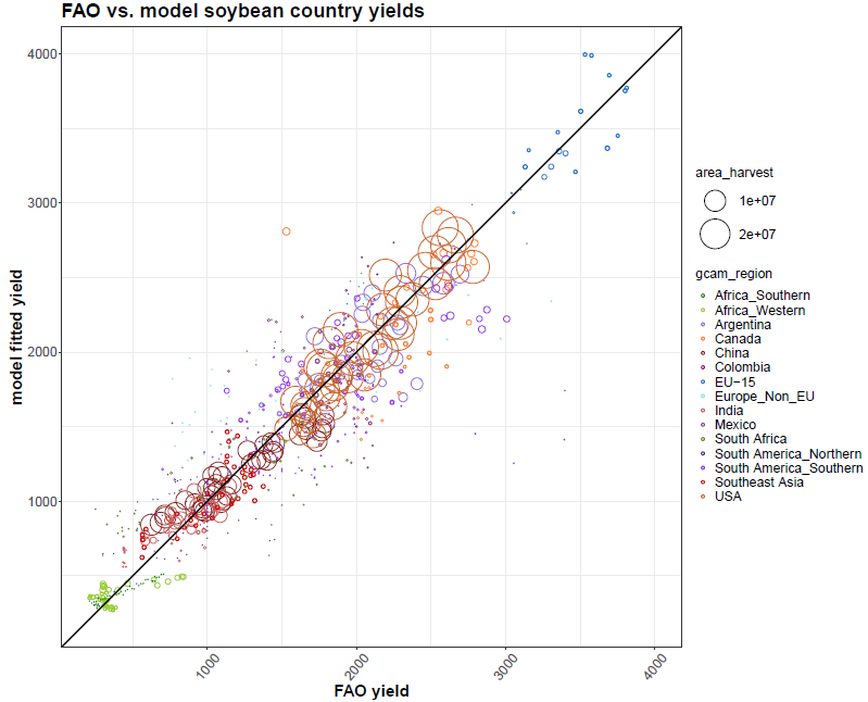
Figure 2: Model fitted yields versus FAO yields for soybean.
yield_shock_projection
Once the gaia model has completed fitting, the
gaia::yield_shock_projection function calculates the
projected annual yield shocks based on the input climate data. The
climate impact on yield, known as yield shock, refers to the fractional
change in a crop’s yield within a specific country during a future
period, relative to the baseline yield that would otherwise obtain under
a stable climate. This concept is mathematically defined in Equations 3
to 6 of Waldhoff et
al., (2020).
For coarse-scale models like GCAM, gaia also computes
smoothed yield shocks using a user-specified smoothing window (the
default window is 20 years). In the smoothed outputs, the yield shocks
at the base year will be set to 1. The results are provided in both
CSV outputs and diagnostic plots.
To run yield_shock_projection, simply pass metadata such
as climate model, climate scenario, base year, start and end year of the
climate data, and smooth window to the function. The code chunk below
shows an example.
# Path to the output folder where you wish to save the outputs. Change it accordingly
output_dir <- 'gaia_example/example_2_output'

# calculate projected yield shocks
out_yield_shock <- yield_shock_projection(use_default_coeff = FALSE,
                                          climate_model = 'canesm5',
                                          climate_scenario = 'ssp245',
                                          base_year = 2015,
                                          start_year = 2015,
                                          end_year = 2100,
                                          smooth_window = 20,
                                          diagnostics = TRUE,
                                          output_dir = output_dir)
Outputs of the function: The
yield_shock_projection function returns a data frame of
formatted smoothed annual crop yield shocks under climate impacts. It
also writes the following output files:
yield_impacts_annual/yield_[climate-model]_[climate-scenario]_[crop-name].csv: This file includes annual crop yield shocks under climate variability. An example of annual soybean yield shocks (column yield_impact) is shown in Table 7.yield_impacts_smooth/yield_[climate-model]_[climate-scenario]_[crop-name].csv: This file includes smoothed annual crop yield shocks under climate variability. The default smoothing window is 20 years. An example of smoothed annual soybean yield shocks is shown in Table 8.annual_projected_climate_impacts_[climate-model]_[climate-scenario]_[crop-name]_[fit-name].pdf: This is diagnostic plot for annual crop yield shocks for countries within different regions. It is located underoutput_dir/figuresfolder. A diagnostic plot of annual soybean yield shocks is illustrated in Figure 3.smooth_projected_climate_impacts_[climate-model]_[climate-scenario]_[crop-name]_[fit-name].pdf: This is diagnostic plot for smoothed annual crop yield shocks for countries within different regions. It is located underoutput_dir/figuresfolder.
The followings are example outputs and diagnostic plot from
yield_shock_projection function.
| GCAM_region_name | iso | crop | year | yield_impact |
|---|---|---|---|---|
| Africa_Southern | tza | soybean | 2015 | 0.9641709 |
| Africa_Western | nga | soybean | 2015 | 0.9474335 |
| Argentina | arg | soybean | 2015 | 0.9698823 |
| Canada | can | soybean | 2015 | 0.9861523 |
| China | chn | soybean | 2015 | 1.0211866 |
| Colombia | col | soybean | 2015 | NA |
| EU-15 | ita | soybean | 2015 | 0.9645651 |
| Europe_Non_EU | tur | soybean | 2015 | 0.9491436 |
| India | ind | soybean | 2015 | 0.8470723 |
| Mexico | mex | soybean | 2015 | 0.9948925 |
| Note: | ||||
| This only shows the first 10 lines of the example data. |
| crop | model | scenario | iso | 2015 | 2016 | 2017 | 2018 | 2019 | 2020 | 2021 | 2022 | 2023 | 2024 | 2025 | 2026 | 2027 | 2028 | 2029 | 2030 | 2031 | 2032 | 2033 | 2034 | 2035 | 2036 | 2037 | 2038 | 2039 | 2040 | 2041 | 2042 | 2043 | 2044 | 2045 | 2046 | 2047 | 2048 | 2049 | 2050 | 2051 | 2052 | 2053 | 2054 | 2055 | 2056 | 2057 | 2058 | 2059 | 2060 | 2061 | 2062 | 2063 | 2064 | 2065 | 2066 | 2067 | 2068 | 2069 | 2070 | 2071 | 2072 | 2073 | 2074 | 2075 | 2076 | 2077 | 2078 | 2079 | 2080 | 2081 | 2082 | 2083 | 2084 | 2085 | 2086 | 2087 | 2088 | 2089 | 2090 | 2091 | 2092 | 2093 | 2094 | 2095 | 2096 | 2097 | 2098 | 2099 | 2100 |
|---|---|---|---|---|---|---|---|---|---|---|---|---|---|---|---|---|---|---|---|---|---|---|---|---|---|---|---|---|---|---|---|---|---|---|---|---|---|---|---|---|---|---|---|---|---|---|---|---|---|---|---|---|---|---|---|---|---|---|---|---|---|---|---|---|---|---|---|---|---|---|---|---|---|---|---|---|---|---|---|---|---|---|---|---|---|---|---|---|---|
| soybean | canesm5 | ssp245 | arg | 1 | 1.0016301 | 1.0032602 | 1.0048903 | 1.0065205 | 1.0081506 | 1.0086019 | 1.0090532 | 1.0095045 | 1.0099559 | 1.0104072 | 1.0108585 | 1.0113098 | 1.0117612 | 1.0122125 | 1.0126638 | 1.0149256 | 1.0171874 | 1.0194492 | 1.0217109 | 1.0239727 | 1.0262345 | 1.0284963 | 1.0307581 | 1.0330198 | 1.0352816 | 1.0362096 | 1.0371375 | 1.0380654 | 1.0389933 | 1.0399213 | 1.0408492 | 1.0417771 | 1.0427051 | 1.0436330 | 1.0445609 | 1.0422303 | 1.0398997 | 1.0375691 | 1.0352385 | 1.0329079 | 1.0305773 | 1.0282468 | 1.0259162 | 1.0235856 | 1.0212550 | 1.0207144 | 1.0201739 | 1.0196334 | 1.0190929 | 1.0185523 | 1.0180118 | 1.0174713 | 1.0169308 | 1.0163902 | 1.0158497 | 1.0193418 | 1.0228339 | 1.0263259 | 1.0298180 | 1.0333101 | 1.0368021 | 1.0402942 | 1.0437863 | 1.0472783 | 1.0507704 | 1.0527891 | 1.0548078 | 1.0568265 | 1.0588452 | 1.0608639 | 1.0628826 | 1.0649013 | 1.0669200 | 1.0689387 | 1.0709574 | 1.0703586 | 1.0697598 | 1.0691610 | 1.0685622 | 1.0679634 | 1.0673647 | 1.0667659 | 1.0661671 | 1.0655683 | 1.0649695 |
| soybean | canesm5 | ssp245 | bol | 1 | 1.0036277 | 1.0072554 | 1.0108832 | 1.0145109 | 1.0181386 | 1.0188126 | 1.0194866 | 1.0201605 | 1.0208345 | 1.0215085 | 1.0221825 | 1.0228564 | 1.0235304 | 1.0242044 | 1.0248784 | 1.0235855 | 1.0222927 | 1.0209999 | 1.0197071 | 1.0184143 | 1.0171215 | 1.0158287 | 1.0145359 | 1.0132431 | 1.0119503 | 1.0112330 | 1.0105156 | 1.0097983 | 1.0090810 | 1.0083637 | 1.0076464 | 1.0069290 | 1.0062117 | 1.0054944 | 1.0047771 | 1.0058617 | 1.0069464 | 1.0080310 | 1.0091156 | 1.0102003 | 1.0112849 | 1.0123696 | 1.0134542 | 1.0145389 | 1.0156235 | 1.0145656 | 1.0135077 | 1.0124498 | 1.0113918 | 1.0103339 | 1.0092760 | 1.0082181 | 1.0071602 | 1.0061023 | 1.0050444 | 1.0036524 | 1.0022605 | 1.0008685 | 0.9994765 | 0.9980846 | 0.9966926 | 0.9953006 | 0.9939087 | 0.9925167 | 0.9911248 | 0.9886305 | 0.9861361 | 0.9836418 | 0.9811475 | 0.9786532 | 0.9761589 | 0.9736646 | 0.9711703 | 0.9686760 | 0.9661817 | 0.9634094 | 0.9606370 | 0.9578646 | 0.9550923 | 0.9523199 | 0.9495476 | 0.9467752 | 0.9440028 | 0.9412305 | 0.9384581 |
| soybean | canesm5 | ssp245 | can | 1 | 1.0000692 | 1.0001383 | 1.0002075 | 1.0002767 | 1.0003459 | 1.0009930 | 1.0016401 | 1.0022873 | 1.0029344 | 1.0035816 | 1.0042287 | 1.0048759 | 1.0055230 | 1.0061702 | 1.0068173 | 1.0085141 | 1.0102109 | 1.0119076 | 1.0136044 | 1.0153012 | 1.0169980 | 1.0186947 | 1.0203915 | 1.0220883 | 1.0237851 | 1.0246978 | 1.0256106 | 1.0265234 | 1.0274362 | 1.0283490 | 1.0292618 | 1.0301745 | 1.0310873 | 1.0320001 | 1.0329129 | 1.0331499 | 1.0333870 | 1.0336240 | 1.0338611 | 1.0340981 | 1.0343352 | 1.0345722 | 1.0348092 | 1.0350463 | 1.0352833 | 1.0333854 | 1.0314875 | 1.0295896 | 1.0276917 | 1.0257938 | 1.0238959 | 1.0219980 | 1.0201001 | 1.0182022 | 1.0163043 | 1.0153924 | 1.0144805 | 1.0135686 | 1.0126567 | 1.0117448 | 1.0108329 | 1.0099210 | 1.0090091 | 1.0080972 | 1.0071853 | 1.0097711 | 1.0123568 | 1.0149426 | 1.0175283 | 1.0201141 | 1.0226998 | 1.0252856 | 1.0278713 | 1.0304571 | 1.0330428 | 1.0343181 | 1.0355934 | 1.0368687 | 1.0381440 | 1.0394193 | 1.0406946 | 1.0419699 | 1.0432452 | 1.0445205 | 1.0457958 |
| soybean | canesm5 | ssp245 | chn | 1 | 1.0067897 | 1.0135794 | 1.0203690 | 1.0271587 | 1.0339484 | 1.0355738 | 1.0371992 | 1.0388246 | 1.0404500 | 1.0420754 | 1.0437009 | 1.0453263 | 1.0469517 | 1.0485771 | 1.0502025 | 1.0511308 | 1.0520592 | 1.0529875 | 1.0539159 | 1.0548442 | 1.0557726 | 1.0567009 | 1.0576293 | 1.0585576 | 1.0594859 | 1.0618462 | 1.0642064 | 1.0665667 | 1.0689269 | 1.0712871 | 1.0736474 | 1.0760076 | 1.0783679 | 1.0807281 | 1.0830884 | 1.0846814 | 1.0862745 | 1.0878676 | 1.0894607 | 1.0910538 | 1.0926469 | 1.0942400 | 1.0958330 | 1.0974261 | 1.0990192 | 1.0995325 | 1.1000457 | 1.1005590 | 1.1010723 | 1.1015855 | 1.1020988 | 1.1026121 | 1.1031253 | 1.1036386 | 1.1041519 | 1.1043906 | 1.1046293 | 1.1048680 | 1.1051066 | 1.1053453 | 1.1055840 | 1.1058227 | 1.1060614 | 1.1063001 | 1.1065388 | 1.1076580 | 1.1087772 | 1.1098964 | 1.1110156 | 1.1121348 | 1.1132541 | 1.1143733 | 1.1154925 | 1.1166117 | 1.1177309 | 1.1183250 | 1.1189192 | 1.1195134 | 1.1201075 | 1.1207017 | 1.1212958 | 1.1218900 | 1.1224841 | 1.1230783 | 1.1236724 |
| soybean | canesm5 | ssp245 | col | 1 | 0.9917471 | 0.9834943 | 0.9752414 | 0.9669885 | 0.9587356 | 0.9533149 | 0.9478941 | 0.9424734 | 0.9370527 | 0.9316319 | 0.9262112 | 0.9207905 | 0.9153697 | 0.9099490 | 0.9045282 | 0.9023201 | 0.9001121 | 0.8979040 | 0.8956959 | 0.8934878 | 0.8912797 | 0.8890716 | 0.8868635 | 0.8846554 | 0.8824473 | 0.8824935 | 0.8825396 | 0.8825858 | 0.8826319 | 0.8826780 | 0.8827242 | 0.8827703 | 0.8828165 | 0.8828626 | 0.8829088 | 0.8844742 | 0.8860396 | 0.8876050 | 0.8891704 | 0.8907358 | 0.8923012 | 0.8938666 | 0.8954320 | 0.8969974 | 0.8985628 | 0.9003042 | 0.9020455 | 0.9037869 | 0.9055282 | 0.9072695 | 0.9090109 | 0.9107522 | 0.9124936 | 0.9142349 | 0.9159763 | 0.9137257 | 0.9114750 | 0.9092244 | 0.9069738 | 0.9047232 | 0.9024726 | 0.9002220 | 0.8979714 | 0.8957207 | 0.8934701 | 0.8920292 | 0.8905883 | 0.8891474 | 0.8877064 | 0.8862655 | 0.8848246 | 0.8833837 | 0.8819428 | 0.8805018 | 0.8790609 | 0.8795957 | 0.8801305 | 0.8806653 | 0.8812002 | 0.8817350 | 0.8822698 | 0.8828046 | 0.8833394 | 0.8838742 | 0.8844090 |
| soybean | canesm5 | ssp245 | guy | 1 | 0.9946807 | 0.9893614 | 0.9840422 | 0.9787229 | 0.9734036 | 0.9700808 | 0.9667579 | 0.9634351 | 0.9601123 | 0.9567895 | 0.9534666 | 0.9501438 | 0.9468210 | 0.9434982 | 0.9401753 | 0.9381465 | 0.9361177 | 0.9340889 | 0.9320601 | 0.9300313 | 0.9280025 | 0.9259737 | 0.9239449 | 0.9219161 | 0.9198873 | 0.9176086 | 0.9153299 | 0.9130512 | 0.9107724 | 0.9084937 | 0.9062150 | 0.9039363 | 0.9016576 | 0.8993789 | 0.8971001 | 0.8976450 | 0.8981899 | 0.8987347 | 0.8992796 | 0.8998245 | 0.9003693 | 0.9009142 | 0.9014591 | 0.9020039 | 0.9025488 | 0.9047994 | 0.9070499 | 0.9093005 | 0.9115510 | 0.9138016 | 0.9160522 | 0.9183027 | 0.9205533 | 0.9228038 | 0.9250544 | 0.9224496 | 0.9198448 | 0.9172399 | 0.9146351 | 0.9120303 | 0.9094255 | 0.9068207 | 0.9042158 | 0.9016110 | 0.8990062 | 0.8973021 | 0.8955980 | 0.8938939 | 0.8921897 | 0.8904856 | 0.8887815 | 0.8870774 | 0.8853733 | 0.8836692 | 0.8819650 | 0.8832957 | 0.8846263 | 0.8859569 | 0.8872875 | 0.8886181 | 0.8899487 | 0.8912794 | 0.8926100 | 0.8939406 | 0.8952712 |
| soybean | canesm5 | ssp245 | ind | 1 | 0.9721613 | 0.9443227 | 0.9164840 | 0.8886453 | 0.8608067 | 0.8503184 | 0.8398301 | 0.8293418 | 0.8188536 | 0.8083653 | 0.7978770 | 0.7873887 | 0.7769004 | 0.7664122 | 0.7559239 | 0.7595445 | 0.7631650 | 0.7667856 | 0.7704062 | 0.7740267 | 0.7776473 | 0.7812679 | 0.7848884 | 0.7885090 | 0.7921296 | 0.7994869 | 0.8068443 | 0.8142017 | 0.8215591 | 0.8289165 | 0.8362739 | 0.8436312 | 0.8509886 | 0.8583460 | 0.8657034 | 0.8841166 | 0.9025298 | 0.9209430 | 0.9393561 | 0.9577693 | 0.9761825 | 0.9945957 | 1.0130089 | 1.0314221 | 1.0498353 | 1.0616913 | 1.0735474 | 1.0854034 | 1.0972595 | 1.1091155 | 1.1209716 | 1.1328276 | 1.1446837 | 1.1565397 | 1.1683958 | 1.1545201 | 1.1406445 | 1.1267688 | 1.1128932 | 1.0990175 | 1.0851418 | 1.0712662 | 1.0573905 | 1.0435149 | 1.0296392 | 1.0164243 | 1.0032094 | 0.9899945 | 0.9767796 | 0.9635647 | 0.9503498 | 0.9371349 | 0.9239200 | 0.9107051 | 0.8974902 | 0.8976492 | 0.8978082 | 0.8979672 | 0.8981262 | 0.8982852 | 0.8984442 | 0.8986032 | 0.8987622 | 0.8989212 | 0.8990802 |
| soybean | canesm5 | ssp245 | ita | 1 | 0.9990641 | 0.9981283 | 0.9971924 | 0.9962565 | 0.9953207 | 0.9954804 | 0.9956401 | 0.9957998 | 0.9959595 | 0.9961192 | 0.9962789 | 0.9964386 | 0.9965983 | 0.9967580 | 0.9969177 | 0.9977259 | 0.9985341 | 0.9993423 | 1.0001505 | 1.0009587 | 1.0017669 | 1.0025750 | 1.0033832 | 1.0041914 | 1.0049996 | 1.0066750 | 1.0083503 | 1.0100256 | 1.0117010 | 1.0133763 | 1.0150516 | 1.0167270 | 1.0184023 | 1.0200777 | 1.0217530 | 1.0215077 | 1.0212624 | 1.0210170 | 1.0207717 | 1.0205264 | 1.0202811 | 1.0200357 | 1.0197904 | 1.0195451 | 1.0192998 | 1.0184871 | 1.0176744 | 1.0168617 | 1.0160491 | 1.0152364 | 1.0144237 | 1.0136110 | 1.0127983 | 1.0119856 | 1.0111730 | 1.0122605 | 1.0133480 | 1.0144356 | 1.0155231 | 1.0166107 | 1.0176982 | 1.0187857 | 1.0198733 | 1.0209608 | 1.0220483 | 1.0229595 | 1.0238707 | 1.0247818 | 1.0256930 | 1.0266042 | 1.0275153 | 1.0284265 | 1.0293377 | 1.0302488 | 1.0311600 | 1.0320589 | 1.0329578 | 1.0338566 | 1.0347555 | 1.0356544 | 1.0365533 | 1.0374522 | 1.0383510 | 1.0392499 | 1.0401488 |
| soybean | canesm5 | ssp245 | mex | 1 | 1.0034726 | 1.0069453 | 1.0104179 | 1.0138906 | 1.0173632 | 1.0180901 | 1.0188170 | 1.0195438 | 1.0202707 | 1.0209976 | 1.0217245 | 1.0224513 | 1.0231782 | 1.0239051 | 1.0246320 | 1.0245834 | 1.0245349 | 1.0244864 | 1.0244378 | 1.0243893 | 1.0243407 | 1.0242922 | 1.0242437 | 1.0241951 | 1.0241466 | 1.0237126 | 1.0232785 | 1.0228445 | 1.0224105 | 1.0219765 | 1.0215425 | 1.0211084 | 1.0206744 | 1.0202404 | 1.0198064 | 1.0203254 | 1.0208445 | 1.0213635 | 1.0218826 | 1.0224016 | 1.0229206 | 1.0234397 | 1.0239587 | 1.0244778 | 1.0249968 | 1.0258074 | 1.0266179 | 1.0274285 | 1.0282390 | 1.0290496 | 1.0298602 | 1.0306707 | 1.0314813 | 1.0322918 | 1.0331024 | 1.0325242 | 1.0319461 | 1.0313679 | 1.0307898 | 1.0302116 | 1.0296335 | 1.0290553 | 1.0284772 | 1.0278990 | 1.0273209 | 1.0273929 | 1.0274650 | 1.0275371 | 1.0276092 | 1.0276812 | 1.0277533 | 1.0278254 | 1.0278975 | 1.0279695 | 1.0280416 | 1.0283166 | 1.0285916 | 1.0288666 | 1.0291417 | 1.0294167 | 1.0296917 | 1.0299667 | 1.0302417 | 1.0305167 | 1.0307917 |
| soybean | canesm5 | ssp245 | nga | 1 | 1.0036285 | 1.0072570 | 1.0108854 | 1.0145139 | 1.0181424 | 1.0212828 | 1.0244233 | 1.0275637 | 1.0307041 | 1.0338446 | 1.0369850 | 1.0401254 | 1.0432659 | 1.0464063 | 1.0495467 | 1.0529853 | 1.0564239 | 1.0598625 | 1.0633011 | 1.0667397 | 1.0701783 | 1.0736169 | 1.0770555 | 1.0804940 | 1.0839326 | 1.0853940 | 1.0868553 | 1.0883167 | 1.0897780 | 1.0912394 | 1.0927007 | 1.0941621 | 1.0956235 | 1.0970848 | 1.0985462 | 1.0975487 | 1.0965513 | 1.0955539 | 1.0945565 | 1.0935590 | 1.0925616 | 1.0915642 | 1.0905668 | 1.0895693 | 1.0885719 | 1.0896377 | 1.0907034 | 1.0917691 | 1.0928349 | 1.0939006 | 1.0949664 | 1.0960321 | 1.0970978 | 1.0981636 | 1.0992293 | 1.1023494 | 1.1054694 | 1.1085895 | 1.1117095 | 1.1148296 | 1.1179496 | 1.1210697 | 1.1241898 | 1.1273098 | 1.1304299 | 1.1309761 | 1.1315224 | 1.1320687 | 1.1326150 | 1.1331613 | 1.1337075 | 1.1342538 | 1.1348001 | 1.1353464 | 1.1358926 | 1.1360448 | 1.1361970 | 1.1363491 | 1.1365013 | 1.1366535 | 1.1368056 | 1.1369578 | 1.1371100 | 1.1372621 | 1.1374143 |
| Note: | |||||||||||||||||||||||||||||||||||||||||||||||||||||||||||||||||||||||||||||||||||||||||
| This only shows the first 10 lines of the example data. |
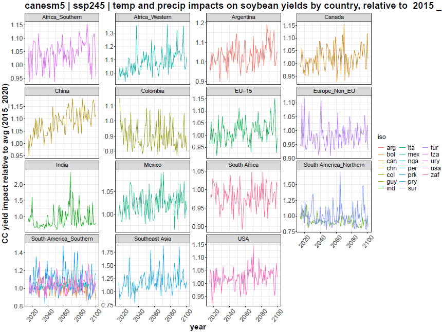
Figure 3: Projected yield shocks for soybean.
gcam_agprodchange
The gcam_agprodchange function is specifically designed
for the Global Change Analysis Model (GCAM) (Calvin et al.,
2019). GCAM requires the agricultural productivity growth rate (APG)
as an input, which is calculated based on yield shocks and the baseline
APG, varying according to different SSP scenarios. Additionally, the APG
for GCAM must be at the region-basin scale. The
gaia::gcam_agprodchange function directly remaps
country-level yield shocks to region-basin APG. In the example below,
since climate_scenario = 'ssp245', it will automatically
pick the baseline APG with SSP2 impact to calculate the climate-impacted
APG based on the yield shocks computed in the previous step. If
climate_scenario is set to other strings that does not
indicate ssp scenario, gaia will use the
baseline APG without any socioeconomic impact.
# Path to the output folder where you wish to save the outputs. Change it accordingly
output_dir <- 'gaia_example/example_2_output'

# calculate region-basin agricultural productivity growth rate for GCAM
gcam_apg <- gcam_agprodchange(data = out_yield_shock,
                              climate_model = 'canesm5',
                              climate_scenario = 'ssp245',
                              member = 'r1i1p1f1',
                              bias_adj = 'w5e5',
                              cfe = 'no-cfe',
                              gcam_version = 'gcam7',
                              diagnostics = TRUE,
                              output_dir = output_dir)
Outputs of the function: The
gcam_agprodchange function returns a data frame of
agricultural productivity change. It also writes the following output
files to the folder named [gcam-version]_agprodchange_[cfe]
(e.g., gcam7_agprodchange_no-cfe):
agyield_impact_[climate-model]_[ensemble-member]_[bias_adj]_[climate-scenario].xml: This is the XML file of agricultural productivity change for all commodities for GCAM.figures_yield_impacts/[commodity.png]: This is diagnostic plot for yield shocks for a GCAM commodity at specifiedgcam_timestep(e.g., 5 years) by basins within each GCAM region (e.g., region-basin intersection) separated by irrigated and rainfed crop types.figures_agprodchange/[commodity.png]: This is diagnostic plot for APG for a GCAM commodity at specifiedgcam_timestep(e.g., 5 years) by basins within each GCAM region (e.g., region-basin intersection) separated by irrigated and rainfed crop types. An example of APG for soybean is shown in Figure 4 below.
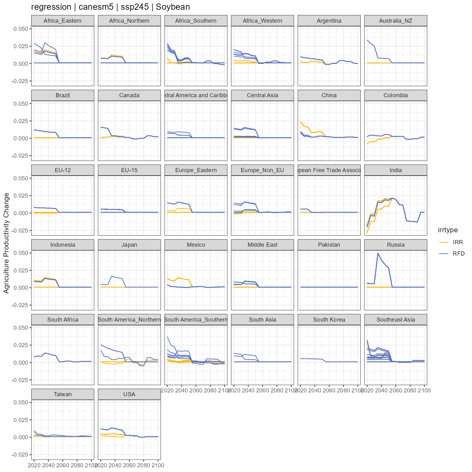
Figure 4: Agricultural productivity growth rate for soybean. Each line under a region indicates the APG for the region-basin intersection.
Limitations
The current version of gaia has several limitations that
users should be aware of.
Weather Data Aggregation and Theoretical Consistency
In the current implementation, gaia uses cropland
area-weighted averages of weather variables (e.g., temperature and
precipitation) to construct country-level climate inputs. While this
aggregation method is commonly used in empirical crop yield modeling,
its theoretical justification is more robust when the dependent variable
(e.g., yield) is in linear form, as it can be interpreted as a
consistent approximation of a field-level data-generating process.
However, in gaia, the dependent variable is specified as
the natural logarithm of yield, which allows us to project the future
yield shocks based on weather only, allowing modelers to use their own
assumptions about technological improvements driving yield improvements.
In this context, the use of cropland-weighted average climate inputs
might lead to theoretical inconsistency. Specifically, if yield is
assumed to be generated by an underlying nonlinear function of weather
at the field level (e.g.,
),
then aggregating climate variables before applying the function is not
equivalent to aggregating yield outcomes after applying the function at
the field level. This is a known issue related to the log-sum-exp
transformation.
While this limitation does not undermine the empirical validity of the model, users should be aware that the aggregation procedure may not be interpretable as a field-level yield formulation. The software currently supports only cropland area-weighted climate and does not offer alternative methods for constructing climate inputs.
Uncertainty Quantification
gaia currently does not explicitly quantify uncertainty
in projected yield shock outcomes resulting from uncertainty in the
estimated econometric coefficients. While gaia provides
statistics of the regression analysis, it does not perform uncertainty
quantification, such as Monte Carlo simulations, to propagate the
uncertainty in model parameters through to the final results. However,
users are provided with all necessary outputs (including coefficient
estimates and associated statistics in the reg_out_[crop]_xxx.csv files)
to implement such an analysis independently, if desired.