Here we visualize the processed data to illustrate the
connection of harvested area and food calories via supply utilization
accounts.
* We focus on the 2013 - 2017 mean as they are the base calibration
years of GCAM. * A user can change the years and mappings as desired. *
All the data used are from gcamfaostat.
* Code for generating the figures are provided in the bottom.
* The visualization here will be continuously updates (suggestions and
pull requests welcome).
* Chord diagram for trade and food processing nests will be added
later.
* We will also try using shiny apps to make them interactive.
Population
Harvested area
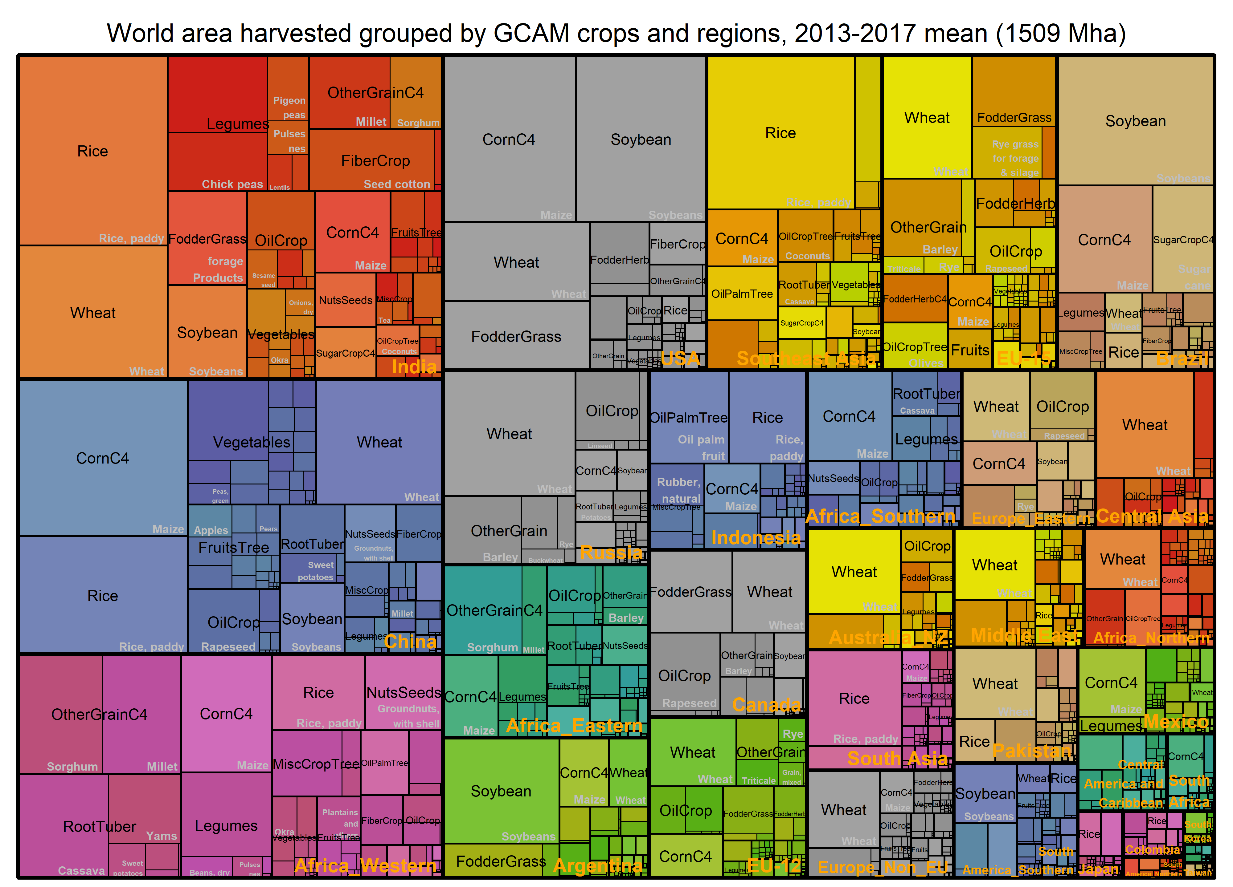
 World area harvested (shares) grouped by GCAM
crops based on the 2013 – 2017 mean values. The total harvested area is
1509 million hectares (Mha).
World area harvested (shares) grouped by GCAM
crops based on the 2013 – 2017 mean values. The total harvested area is
1509 million hectares (Mha).
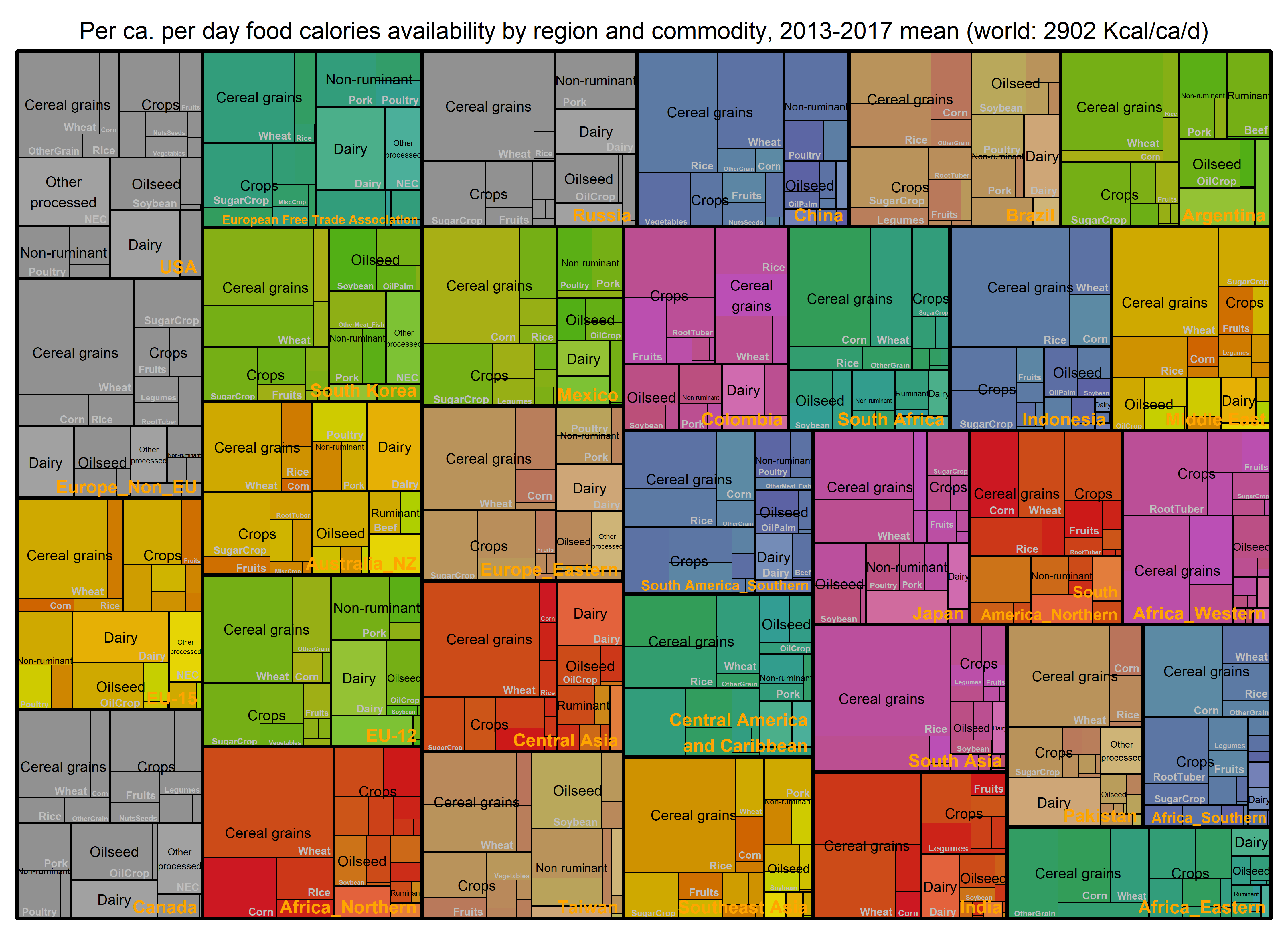
 Food calories availability per capita per day
grouped by GCAM regions and commodities based on the 2013 – 2017 mean
values. The world average value is 2902 Kcal per capita per day
(Kcal/ca/d).
Food calories availability per capita per day
grouped by GCAM regions and commodities based on the 2013 – 2017 mean
values. The world average value is 2902 Kcal per capita per day
(Kcal/ca/d).
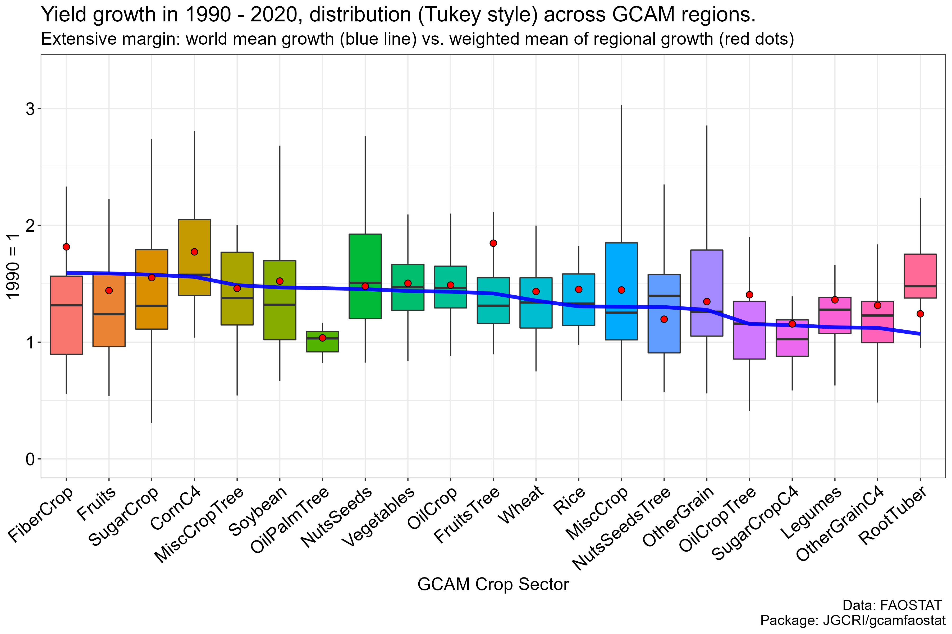
Yield growth
Supply-utilization
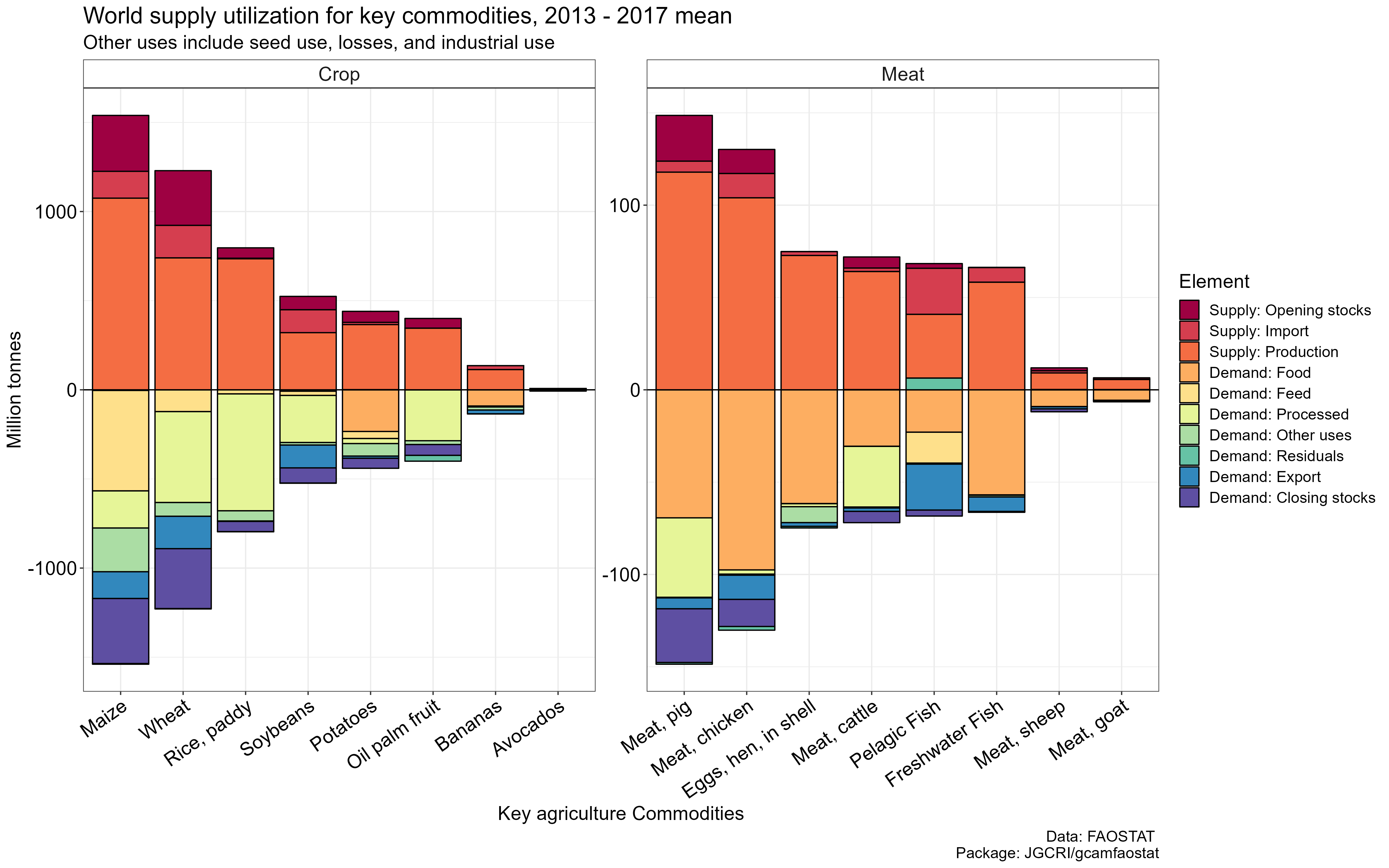 World supply utilization accounts for key commodities based on the 2013
– 2017 mean values. Note that negative values are used for demand
categories and positive values are used for supply categories. Other
uses include seed use, losses, and industrial use; residuals (mostly
small) indicate the imbalance in the data, mainly implying the quality
of the source data. The total supply is equal to the total demand.
World supply utilization accounts for key commodities based on the 2013
– 2017 mean values. Note that negative values are used for demand
categories and positive values are used for supply categories. Other
uses include seed use, losses, and industrial use; residuals (mostly
small) indicate the imbalance in the data, mainly implying the quality
of the source data. The total supply is equal to the total demand.
Code for generating figures
0. Load package data
- Load gcamfaostat locally, assuming driver_drake() was run so that data can be loaded from cache.
devtools::load_all()
# Load other libraries
library(ggplot2)
library(dplyr)
library(treemap)
library(RColorBrewer)

## Define input data needed ----
MODULE_INPUTS <-
  c(FILE = "aglu/FAO/FAO_ag_items_PRODSTAT",
    FILE = "common/GCAM_region_names",
    FILE = "common/iso_GCAM_regID",
    FILE = "aglu/AGLU_ctry",
    "FAO_Food_Macronutrient_All_2010_2019",
    "QCL_CROP_PRIMARY",
    "QCL_FODDERCROP",
    "Bal_new_all",
"OA")- To get more information of the input data and trace their use in the
package, use
infoordstracefunction. They are functions inherited fromgcamdatafor tracing data processing flows.
- Load the data defined in
MODULE_INPUTSfrom drake cache
# Load the data to all_data as a list
MODULE_INPUTS %>% load_from_cache() -> all_data
# Assign the data items to their names as data frames
get_data_list(all_data, MODULE_INPUTS, strip_attributes = TRUE)- Define a base year period for visualizing cross-sectional data. The mean value will be used. Note that 2013-2017 is used here since 2015 is the GCAM v7 base year. However, this can be changed to other year(s)
BaseYear <- c(2013:2017)1. Population
- Get data ready
# simplify population data
OA %>% filter(element_code == 511, item_code == 3010) %>%
  transmute(area, area_code, year, value = value / length(BaseYear)) %>%
  filter(year %in% BaseYear) %>%
  gcamdata::left_join_error_no_match(AGLU_ctry %>% select(area = FAO_country, iso), by = "area") %>%
  gcamdata::left_join_error_no_match(iso_GCAM_regID %>% select(iso, GCAM_region_ID), by = "iso") %>%
  left_join(GCAM_region_names, by = "GCAM_region_ID") ->
POP #1000 persons- Plot and save
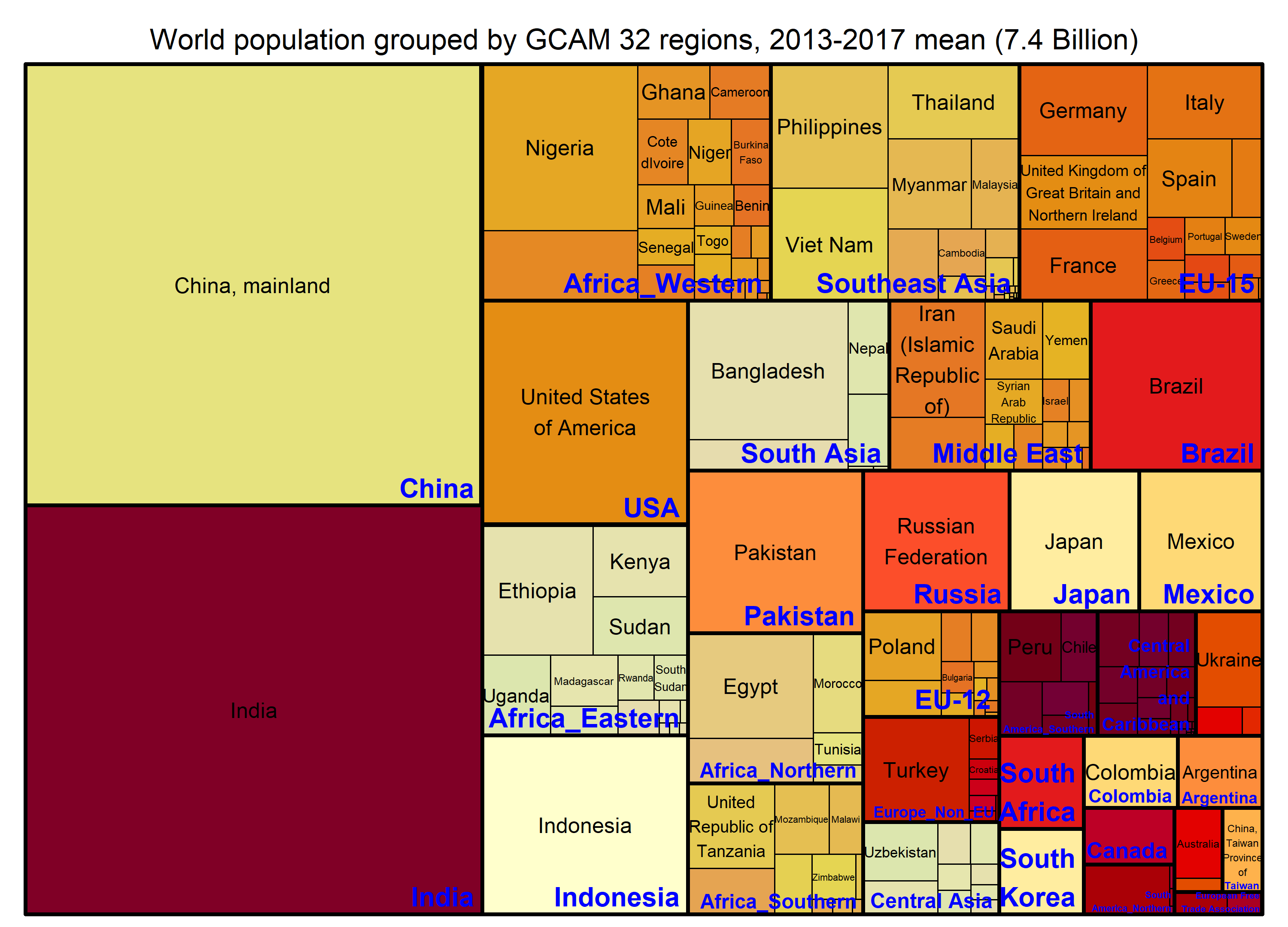
# Figure title
paste0("World population grouped by GCAM 32 regions, ", min(BaseYear), "-", max(BaseYear), " mean (",
       round(POP %>% summarize(value = sum(value) / 1000000),1), " Billion)") -> title

treemap_wrapper(
  .DF = POP %>% select(region, area, value),
  .Depth = 2,
  .Palette = "YlOrRd", .LastLabelCol = "blue",
  .FigTitle = title, .FigTitleSize = 16,
  .SaveName = "Fig_WorldPopulation",
  .SaveScaler = 1.2
)- Preview
2. Harvested area
- Get data ready
QCL_CROP_PRIMARY %>%
  bind_rows(QCL_FODDERCROP) %>%
  filter(year %in% BaseYear) %>%
  filter(element == "Area harvested") %>%
  # Change to Mha
  mutate(value = value / 1000000) %>% select(-unit) %>%
  # the iso mapping in AGLU_ctry works good now
  gcamdata::left_join_error_no_match(AGLU_ctry %>% select(area = FAO_country, iso), by = "area") %>%
  gcamdata::left_join_error_no_match(iso_GCAM_regID %>% select(iso, GCAM_region_ID), by = "iso") %>%
  left_join(GCAM_region_names, by = "GCAM_region_ID") %>%
  group_by(region, item_code, item) %>%
  # 5-year average
  summarize(value = sum(value) / length(BaseYear), .groups = "drop") %>%
  ungroup() %>%
  inner_join(
    FAO_ag_items_PRODSTAT %>%
      filter(!is.na(item), !is.na(GCAM_commodity)) %>%
      select(item_code, GCAM_subsector), by = "item_code") ->
Tree_Area_Reg_Sector- Plot and save
paste0("World area harvested grouped by GCAM crops, ", min(BaseYear), "-", max(BaseYear), " mean (",
       round(Tree_Area_Reg_Sector %>% summarize(value = sum(value) ),0), " Mha)") -> title

treemap_wrapper(
  .DF = Tree_Area_Reg_Sector %>% select(GCAM_subsector, item, value),
  .Depth = 2,
  .Palette = "Set2",
  .FigTitle = title, .FigTitleSize = 16,
  .SaveName = "Fig_WorldAreaHarvested",
  .SaveScaler = 1.1
)

paste0("World area harvested grouped by GCAM crops and regions, ", min(BaseYear), "-", max(BaseYear), " mean (",
       round(Tree_Area_Reg_Sector %>% summarize(value = sum(value) ),0), " Mha)") -> title

treemap_wrapper(
  .DF = Tree_Area_Reg_Sector %>% select(region, GCAM_subsector, item, value),
  .Depth = 3,
  .Palette = "Set2",
  .FigTitle = title, .FigTitleSize = 20,
  .SaveName = "Fig_WorldAreaHarvestedReg",
  .SaveScaler = 1.6
)- Preview
3. Yield
- Get data ready
YieldBaseYear = 1990
QCL_CROP_PRIMARY %>%
  # disaggregate dissolved regions in history
  FAO_AREA_DISAGGREGATE_HIST_DISSOLUTION_ALL(SUDAN2012_MERGE = T) %>%
  # the iso mapping in AGLU_ctry works good now
  left_join_error_no_match(AGLU_ctry %>% select(area = FAO_country, iso), by = "area") %>%
  left_join_error_no_match(iso_GCAM_regID %>% select(iso, GCAM_region_ID), by = "iso") %>%
  left_join(GCAM_region_names, by = "GCAM_region_ID") %>%
  group_by(GCAM_region_ID, region, element, unit, year, item_code) %>%
  # aggregate to 32 GCAM regions
  summarize(value = sum(value), .groups = "drop") %>%
  inner_join(
    FAO_ag_items_PRODSTAT %>%
      filter(!is.na(item), !is.na(GCAM_commodity)) %>%
      select(item_code, GCAM_subsector), by = "item_code") %>%
  group_by_at(vars(GCAM_region_ID, region, GCAM_subsector, year, element)) %>%
  # Aggregate to GCAM sectors
  summarize(value = sum(value), .groups = "drop") %>%
  filter(year %in% c(YieldBaseYear, 2020)) %>%
  spread(element, value) %>%
  filter(`Area harvested` > 0) %>%
  # Calculate regio-sector yield
  mutate(Yield = Production / `Area harvested`) %>%
  gather(element, value, `Area harvested`, Production,  Yield) ->
  Yield_1990_2020_GCAMRegSector

Yield_1990_2020_GCAMRegSector %>%
  filter(element == "Yield") %>%
  group_by_at(vars(-year, -value)) %>%
  # Calculate growth rate
  mutate(value = value / first(value)) %>%
  filter(!is.na(value)) %>%  filter(year != YieldBaseYear) ->
  Yield_1990_2020_GCAMRegSector_Growth

Yield_1990_2020_GCAMRegSector_Growth %>%
  # Join area to get weight
  left_join_error_no_match(Yield_1990_2020_GCAMRegSector %>%
                             filter(element == "Area harvested") %>% spread(element, value),
                           by = c("GCAM_region_ID", "region", "GCAM_subsector", "year")) %>%
  group_by_at(vars(GCAM_subsector, year)) %>%
  summarize(value = weighted.mean(value, w = `Area harvested`), .groups = "drop")->
  Yield_1990_2020_WorldGCAMSector_Growth_FixdArea

Yield_1990_2020_GCAMRegSector %>%
  spread(element, value) %>%
  group_by_at(vars(GCAM_subsector, year)) %>%
  summarize(Production = sum(Production),
         `Area harvested` = sum(`Area harvested`), .groups = "drop") %>%
  mutate(Yield = Production / `Area harvested`) %>%
  gather(element, value, `Area harvested`, Production,  Yield) %>%
  filter(element == "Yield") %>%
  group_by_at(vars(-year, -value)) %>%
  mutate(value = value / first(value)) %>%
  filter(!is.na(value)) %>%  filter(year != YieldBaseYear) ->
  Yield_1990_2020_WorldGCAMSector_Growth_ChangingArea

# Order sectors
Yield_1990_2020_WorldGCAMSector_Growth_ChangingArea%>%
arrange(-value) %>% pull(GCAM_subsector) -> SectorRank- Plot and save
Yield_1990_2020_GCAMRegSector_Growth %>%
  mutate(GCAM_subsector = factor(GCAM_subsector, levels = SectorRank)) %>%
  ggplot() +
  geom_boxplot(aes(x = GCAM_subsector, y = value, fill = GCAM_subsector), outlier.size = -1) +
  geom_line(data = Yield_1990_2020_WorldGCAMSector_Growth_ChangingArea %>%
              mutate(GCAM_subsector = factor(GCAM_subsector, levels = SectorRank)),
             aes(x = GCAM_subsector, y = value, group = year), color = "blue", size = 1.6, alpha = 0.9 ) +
  geom_point(data = Yield_1990_2020_WorldGCAMSector_Growth_FixdArea,
             aes(x = GCAM_subsector, y = value), fill = "red", size = 2.5, shape = 21, color = "black" ) +
  scale_y_continuous(limits = c(0, 3.3)) +
  labs(y = "1990 = 1", x = "GCAM Crop Sector",
       title = "Yield change in 1990 - 2020, distribution (Tukey style) across GCAM regions.",
       subtitle = "World mean growth (blue line) vs. weighted mean of regional growth (red dots)",
       caption = "Data: FAOSTAT \n Package: JGCRI/gcamfaostat") +
  theme_bw() +
  theme(text = element_text(size = 16),
        axis.text = element_text(colour = "black", size = 16),
        axis.text.x = element_text(angle = 40, hjust = 1, vjust = 1),
        strip.background = element_rect(fill = "grey90"),
        legend.position = "none") -> p

ggsave(file.path("../man/figures", "WorldYield.png"), p, width = 15, height = 10)- Preview
4. Supply-utilization
- Get data ready
# Define elements and items
c("Opening stocks", "Import", "Production") -> ElEMSupply
c("Food", "Feed",  "Processed", "Other uses", "Export", "Closing stocks", "Residuals") -> ELEMDemand
c(ElEMSupply, ELEMDemand) -> ELEMAll

c(ElEMSupply, ELEMDemand %>% rev) -> ELEMLevel
c(paste0("Supply: ", ElEMSupply), paste0("Demand: ", ELEMDemand) %>% rev ) -> ELEMLabel
c("Maize", "Wheat", "Rice, paddy", "Soybeans", "Potatoes", "Oil palm fruit", "Bananas", "Avocados") -> KeySectorCrops

# These are items from FAO
c("Meat, pig", "Meat, chicken", "Eggs, hen, in shell", "Meat, cattle",
  "Pelagic Fish", "Freshwater Fish" , "Meat, sheep", "Meat, goat") -> KeySectorMeat
c(KeySectorCrops, KeySectorMeat) -> SECLevel

# Define color pal.
c(brewer.pal(n = length(ELEMAll), name = "Spectral")[1:length(ElEMSupply)],
  brewer.pal(n = length(ELEMAll), name = "Spectral")[length(ElEMSupply)+1:length(ELEMDemand)]
) -> ColUpdate


Bal_new_all %>%
  filter(year %in% BaseYear) %>%
  # Aggregate seed and loss into others
  mutate(element = replace(element, element %in% c("Seed", "Loss"), "Other uses")) %>%
  group_by_at(vars(-value, -area_code, -area)) %>%
  summarize(value = sum(value) / 1000, .groups = "drop") %>%
  filter(element %in% ELEMAll, item %in% SECLevel) %>%
  # year-average
  group_by_at(vars(-value, -year)) %>%
  summarize(value = mean(value), .groups = "drop") %>%
  mutate(value = if_else(!element %in% ElEMSupply, -value, value)) %>%
  mutate(element = factor(element, levels = ELEMLevel, labels = ELEMLabel),
         item = factor(item, levels = SECLevel, labels = SECLevel)) %>%
  mutate(CropMeat = if_else(item %in% KeySectorCrops, "Crop", "Meat")) ->
DF_SUA- Plot and save
DF_SUA %>%
  ggplot() + facet_wrap(~CropMeat, scales = "free") +
    geom_bar(aes(x = item, y = value, fill = element),
             stat = "identity", color = "black", position="stack") +
  geom_hline(yintercept = 0)+
  scale_fill_manual(values = c("Supply: Opening stocks" = ColUpdate[1],
                               "Supply: Import" = ColUpdate[2],
                               "Supply: Production" = ColUpdate[3],
                               "Demand: Food" = ColUpdate[4],
                               "Demand: Feed" = ColUpdate[5],
                               "Demand: Processed" = ColUpdate[6],
                               "Demand: Other uses" = ColUpdate[7],
                               "Demand: Residuals" = ColUpdate[8],
                               "Demand: Export" = ColUpdate[9],
                               "Demand: Closing stocks" = ColUpdate[10] ) ) +
  labs(x = "Key agriculture Commodities",
       y = "Million tonnes", fill = "Element",
       title = "World supply utilization for key commodities, 2013 - 2017 mean",
       subtitle = "Other uses include seed use, losses, and industrial use",
       caption = "Data: FAOSTAT \n Package: JGCRI/gcamfaostat") +
  theme_bw() +
  theme(text = element_text(size = 16),
        axis.text = element_text(colour = "black", size = 16),
        axis.text.x = element_text(angle = 35, hjust = 1, vjust = 1),
        strip.background = element_rect(fill = "grey100"),
        strip.text = element_text(size = 16)) -> p;p

ggsave(file.path("../man/figures", "Fig_WorldSUA.png"), p, width = 16, height = 10)- Preview
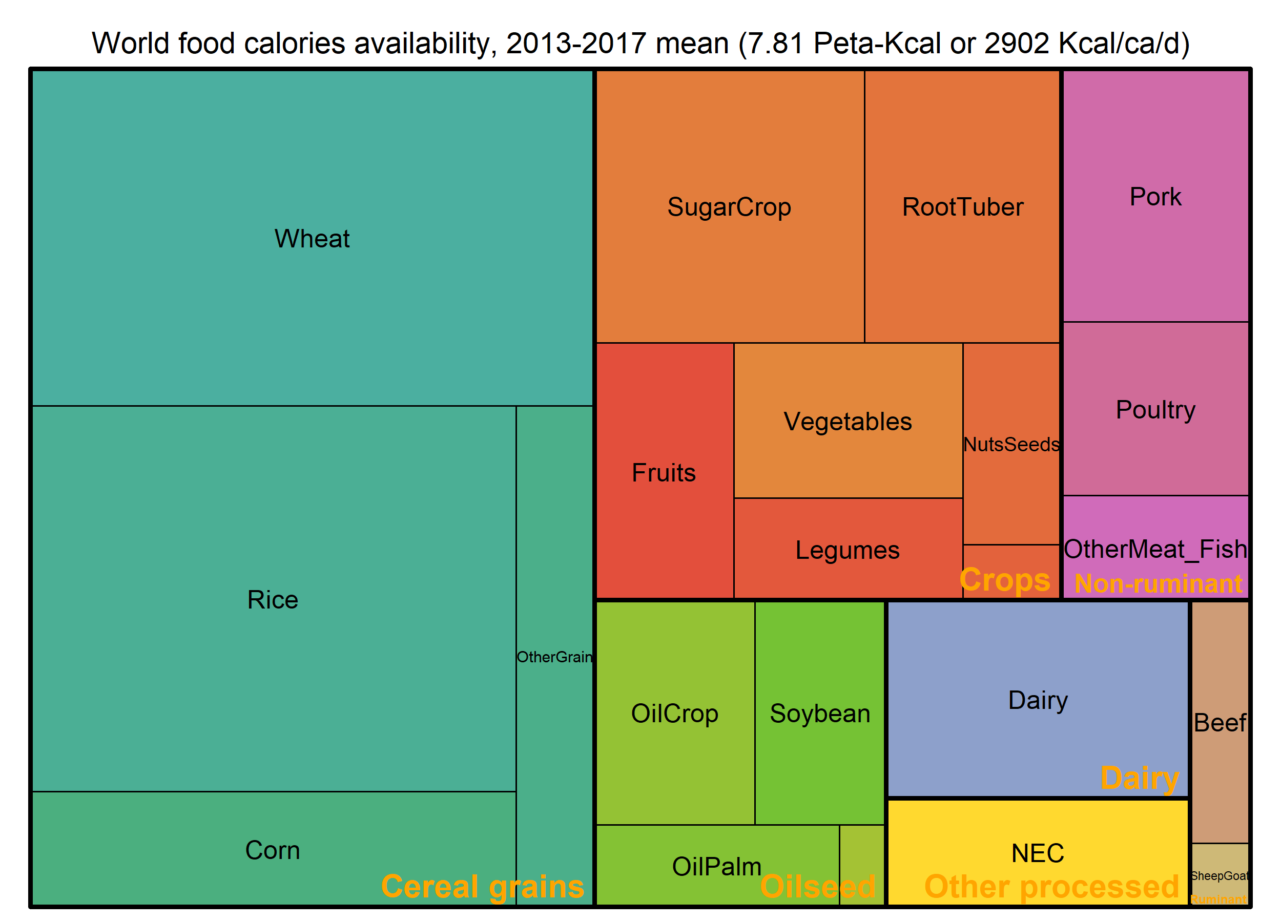
5. Food calories
- Get data ready
FAO_Food_Macronutrient_All_2010_2019 %>%
  filter(year %in% BaseYear) %>%
  # Aggregate to region and GCAM commodity
  dplyr::group_by_at(vars(GCAM_region_ID, GCAM_commodity, year, macronutrient)) %>%
  summarise(value = sum(value), .groups = "drop") %>%
  # Mean over aglu.MODEL_MACRONUTRIENT_YEARS
  dplyr::group_by_at(vars(-year, -value)) %>%
  summarise(value = mean(value), .groups = "drop") %>%
  spread(macronutrient, value) %>%
  left_join_error_no_match(
    POP %>% group_by(GCAM_region_ID, region) %>%
      summarize(POP = sum(value)/1000, .groups = "drop"), # Million
    by = "GCAM_region_ID"
  ) %>%
  # Grouping
  mutate(MeatCrop = if_else(GCAM_commodity %in%
                              c("Beef", "SheepGoat", "Dairy", "OtherMeat_Fish", "Pork", "Poultry"), "Meat", "Crop")) %>%
  mutate(Food = if_else(GCAM_commodity %in%
                          c("Beef", "SheepGoat"), "Ruminant", "Crops"),
         Food = if_else(GCAM_commodity %in%  c("OtherMeat_Fish", "Pork", "Poultry"),
                        "Non-ruminant", Food),
         Food = if_else(GCAM_commodity %in%  c("Dairy"),
                        "Dairy", Food),
         Food = if_else(GCAM_commodity %in% "NEC", "Other processed", Food),
         Food = if_else(GCAM_commodity %in% c("OilCrop", "Soybean", "OilPalm",  "FiberCrop"), "Oilseed", Food),
         Food = if_else(GCAM_commodity %in% c("Corn", "Wheat", "Rice", "OtherGrain"), "Cereal grains", Food)) %>%
  mutate(PcPdKcal = MKcal / POP / 365) ->
DF_Macronutrient_FoodItem- Plot and save
DF_Macronutrient_FoodItem %>%
summarize(PKcal = sum(MKcal)/10^9) %>%
left_join(POP %>% summarize(BPOP = sum(value) / 1000000), by = character()) %>%
mutate(PcPdKcal = PKcal / BPOP / 365 * 1000000) -> WorldSTAT
# World level by commodity
paste0("World food calories availability, ", min(BaseYear), "-", max(BaseYear), " mean (",
round(WorldSTAT$PKcal,2), " Peta-Kcal or ", round(WorldSTAT$PcPdKcal, 0)," Kcal/ca/d)") ->
title
treemap_wrapper(
.DF = DF_Macronutrient_FoodItem %>% select(Food, GCAM_commodity, value = MKcal),
.Depth = 2,
.FigTitle = title, .FigTitleSize = 14,
.SaveName = "Fig_WorldFoodCalories",
.SaveScaler = 1
)
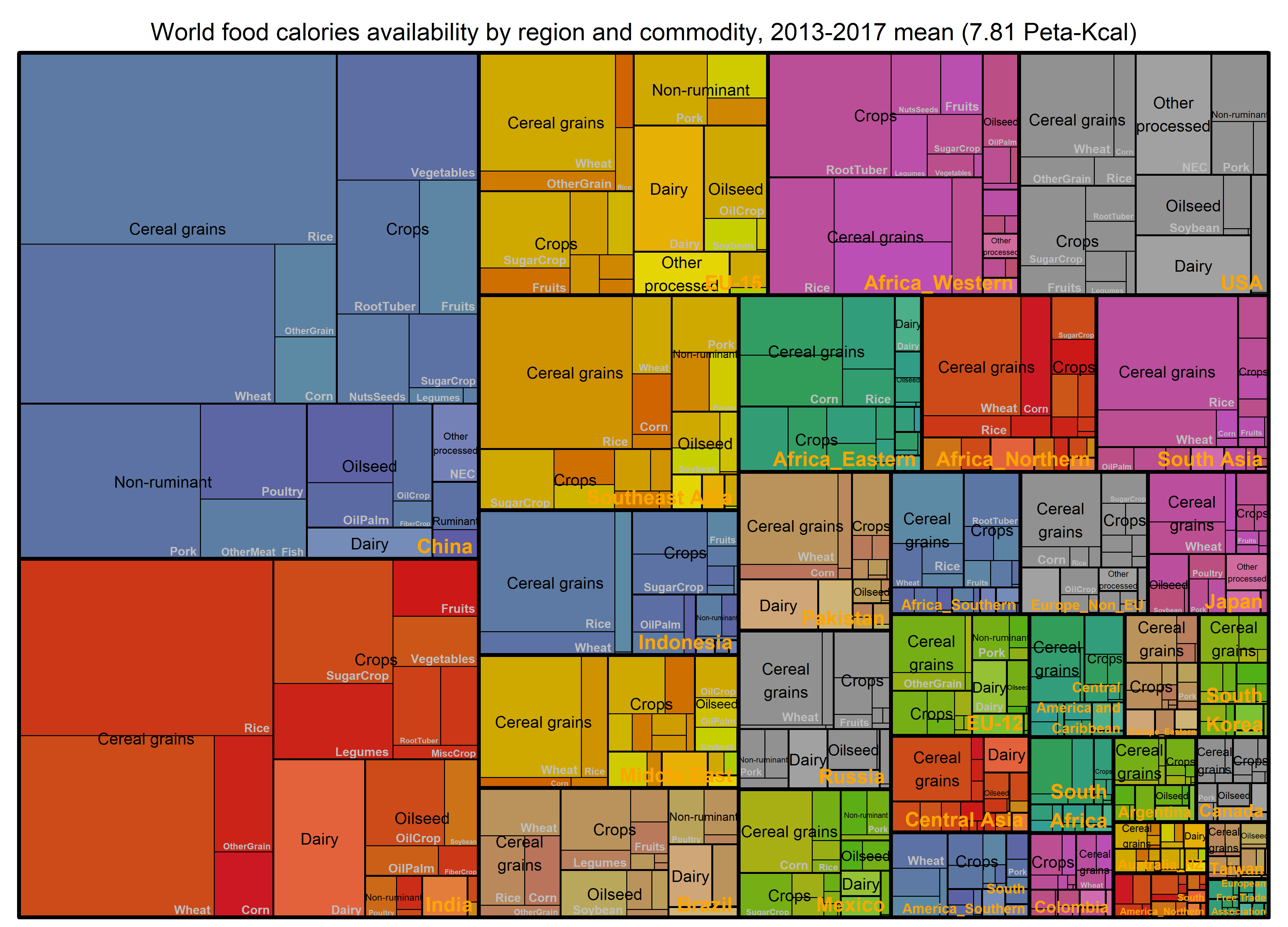
# By commodity and region
paste0("World food calories availability by region and commodity, ", min(BaseYear), "-", max(BaseYear), " mean (",
round(WorldSTAT$PKcal,2), " Peta-Kcal)") ->
title
treemap_wrapper(
.DF = DF_Macronutrient_FoodItem %>% select(region, Food, GCAM_commodity, value = MKcal),
.Depth = 3,
.FigTitle = title, .FigTitleSize = 18,
.SaveName = "Fig_WorldFoodCaloriesReg",
.SaveScaler = 1.6
)
# By commodity and region per ca per day
paste0("Per ca. per day food calories availability by region and commodity, ",
min(BaseYear), "-", max(BaseYear), " mean (world: ", round(WorldSTAT$PcPdKcal, 0)," Kcal/ca/d)") ->
title
treemap_wrapper(
.DF = DF_Macronutrient_FoodItem %>% select(region, Food, GCAM_commodity, value = PcPdKcal),
.Depth = 3,
.FigTitle = title, .FigTitleSize = 20,
.SaveName = "Fig_WorldFoodCaloriesRegPcPerDay",
.SaveScaler = 1.8
)- Preview
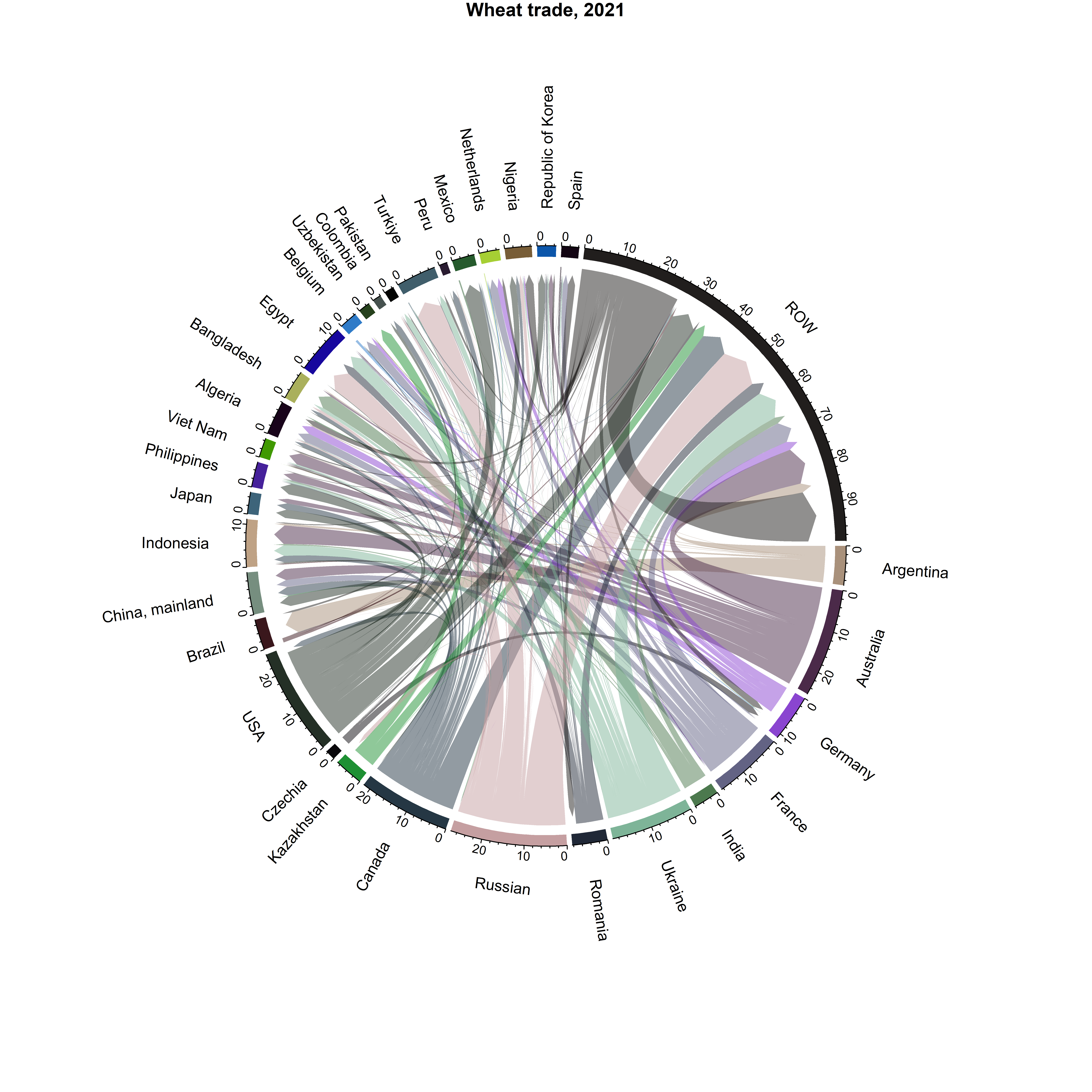
6. Trade
See Cast Study for details.