Key Links

Github: https://github.com/JGCRI/metis
Webpage: https://jgcri.github.io/metis/
Cheatsheet: https://github.com/JGCRI/metis/blob/master/metisCheatsheet.pdf

Folder Structure & Inputs

Folder structure

Key inputs

Maps Available

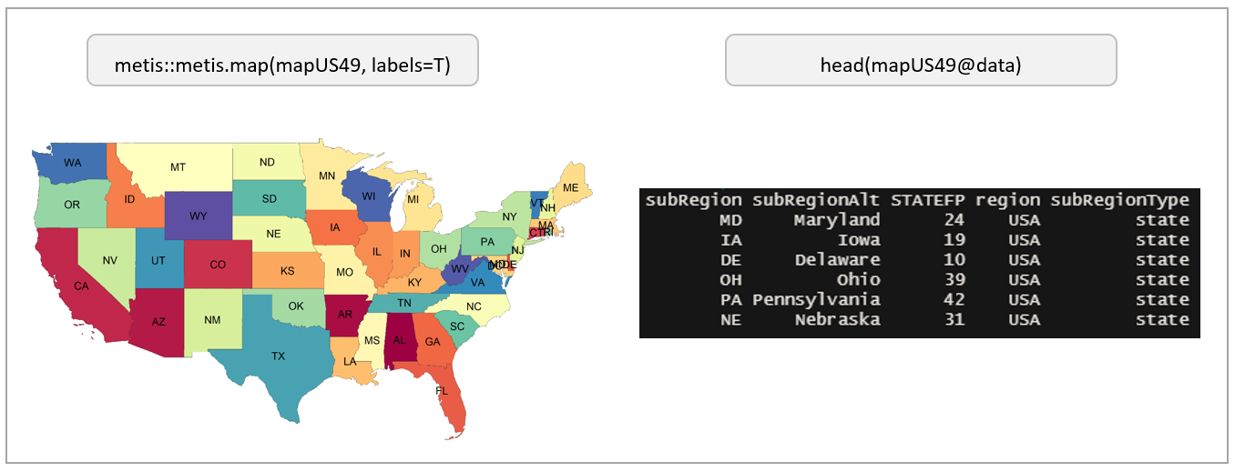
Metis comes with a set of preloaded maps. A full list of metis maps is available at colors, maps and params. The pre-loaded maps all come with each polygon labelled in a subRegion column. For each map the data contained in the shapefile and the map itself can be viewed as follows:

library(metis)

head(mapUS49@data) # To View data in shapefile
metis::metis.map(mapUS49, labels=T)

Example View of Pre-loaded Map for US49

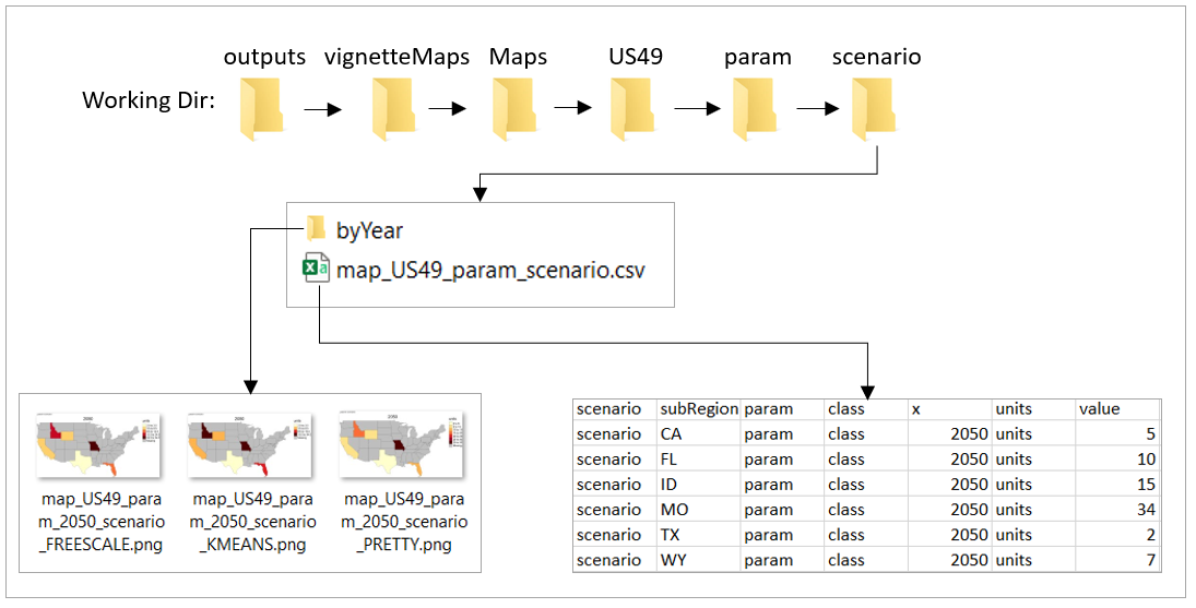
Plot Data on Maps

Auto Map Find

metis.mapsProcess will search through the list of pre-loaded metis maps to see if it can find the “subRegions” provided in the data and then plot the data on those maps. Some examples are provided below:

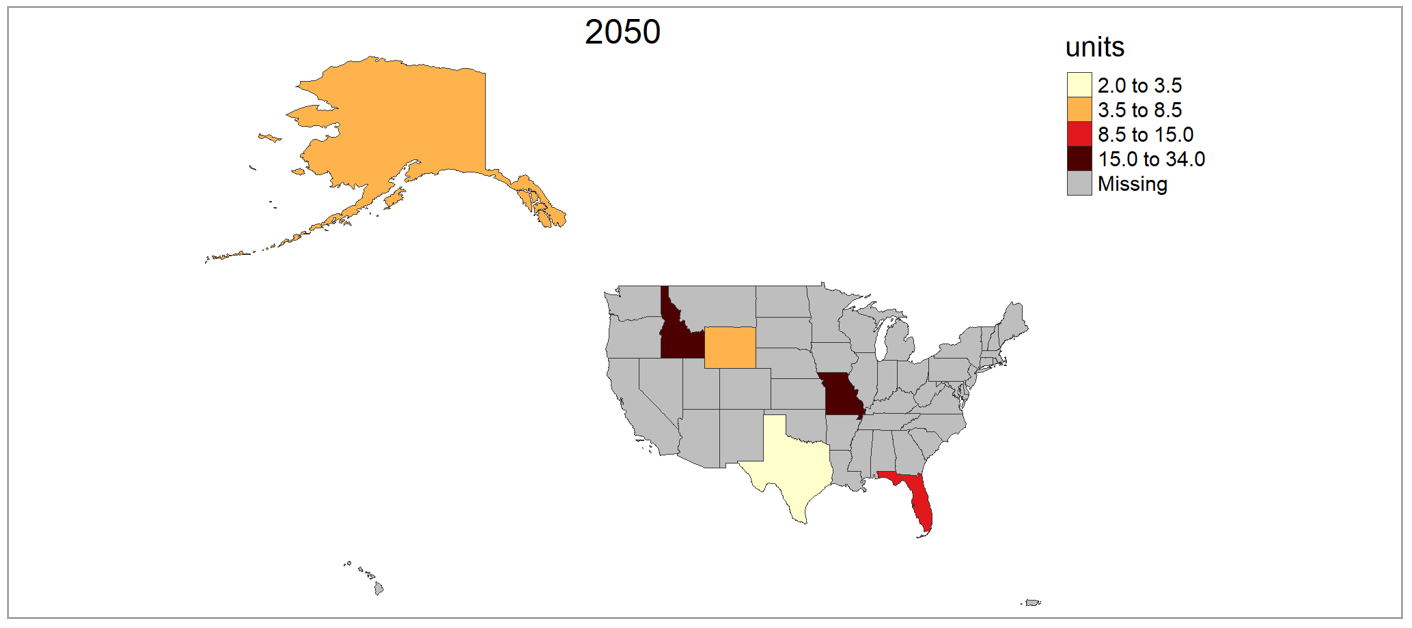
US 49

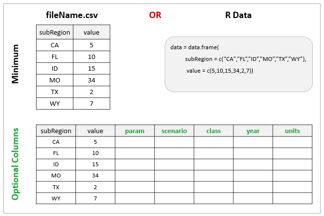
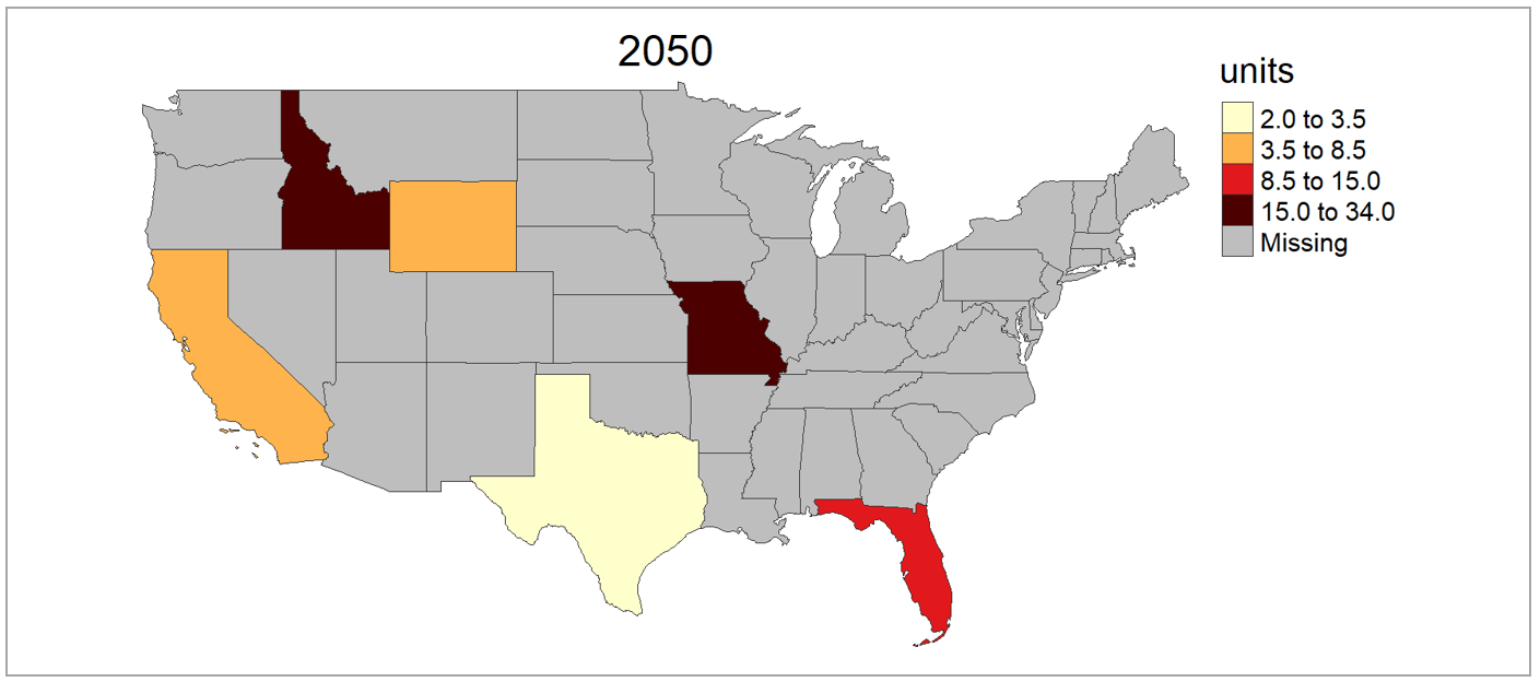
library(metis)

data = data.frame(subRegion=c("CA","FL","ID","MO","TX","WY"),
                  x=c(2050,2050,2050,2050,2050,2050),
                  value=c(5,10,15,34,2,7))
metis.mapsProcess(polygonTable=data,
                  folderName = "vignetteMaps", mapTitleOn = F)

US49

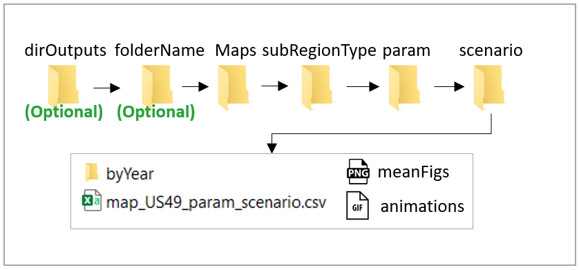
US49 Outputs structure

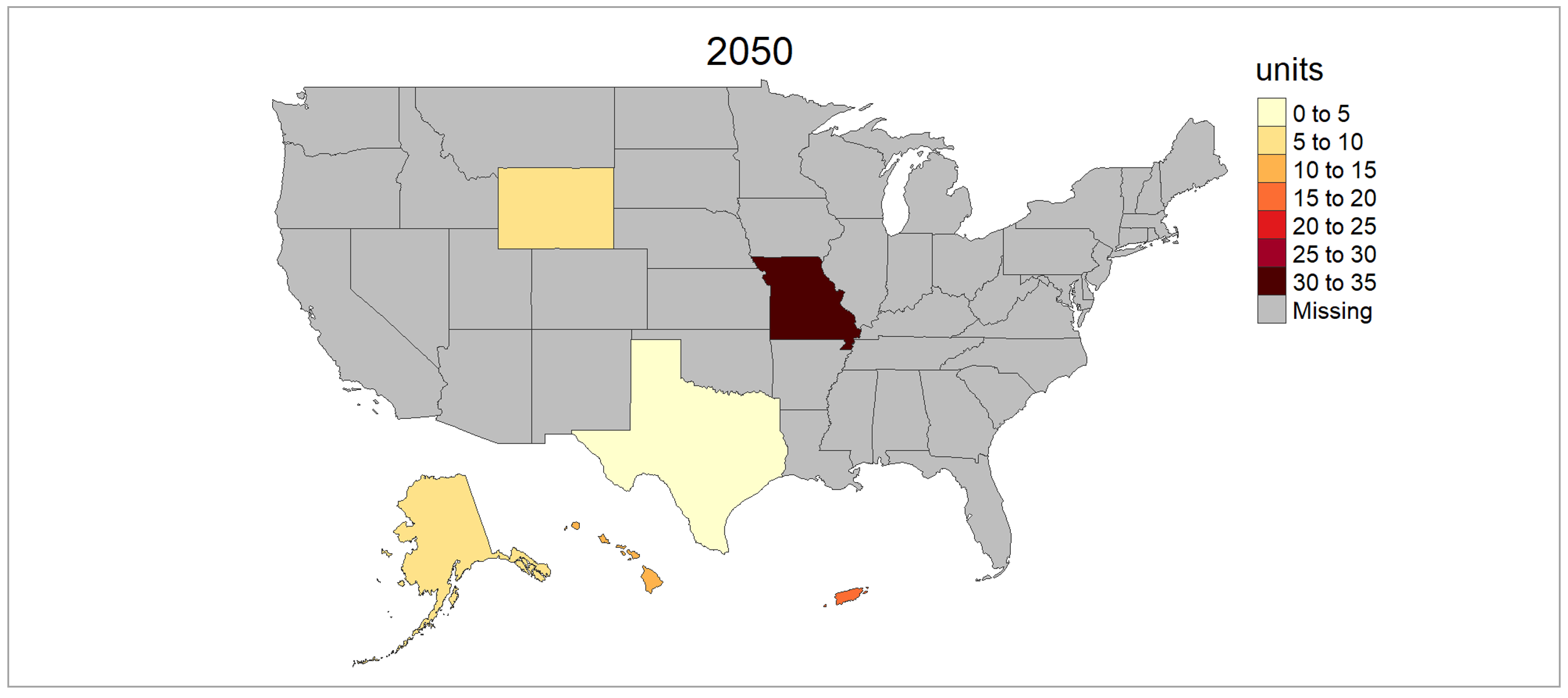
US 52

library(metis)

data = data.frame(subRegion=c("AK","FL","ID","MO","TX","WY"),
                  x=c(2050,2050,2050,2050,2050,2050),
                  value=c(5,10,15,34,2,7))
metis.mapsProcess(polygonTable=data,
                  folderName = "vignetteMaps", mapTitleOn = F)

US52

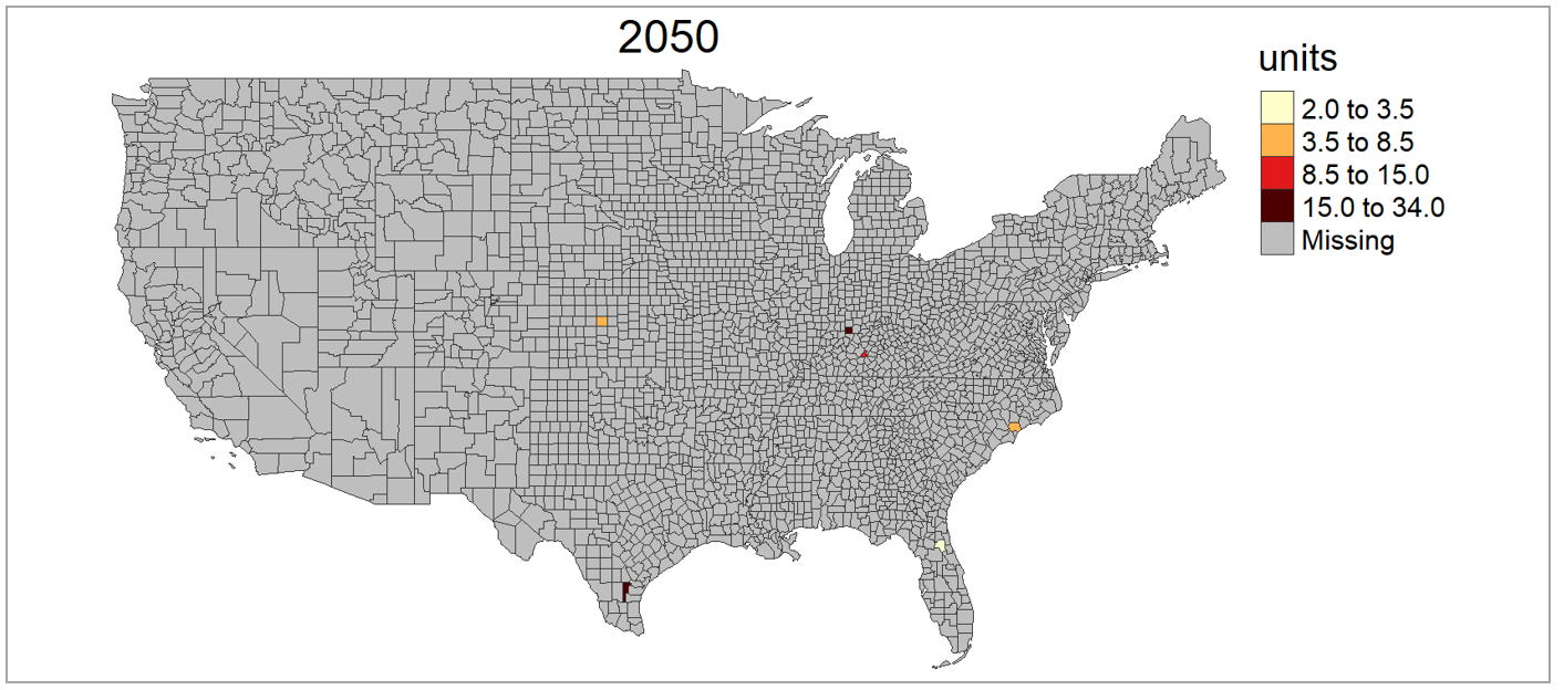
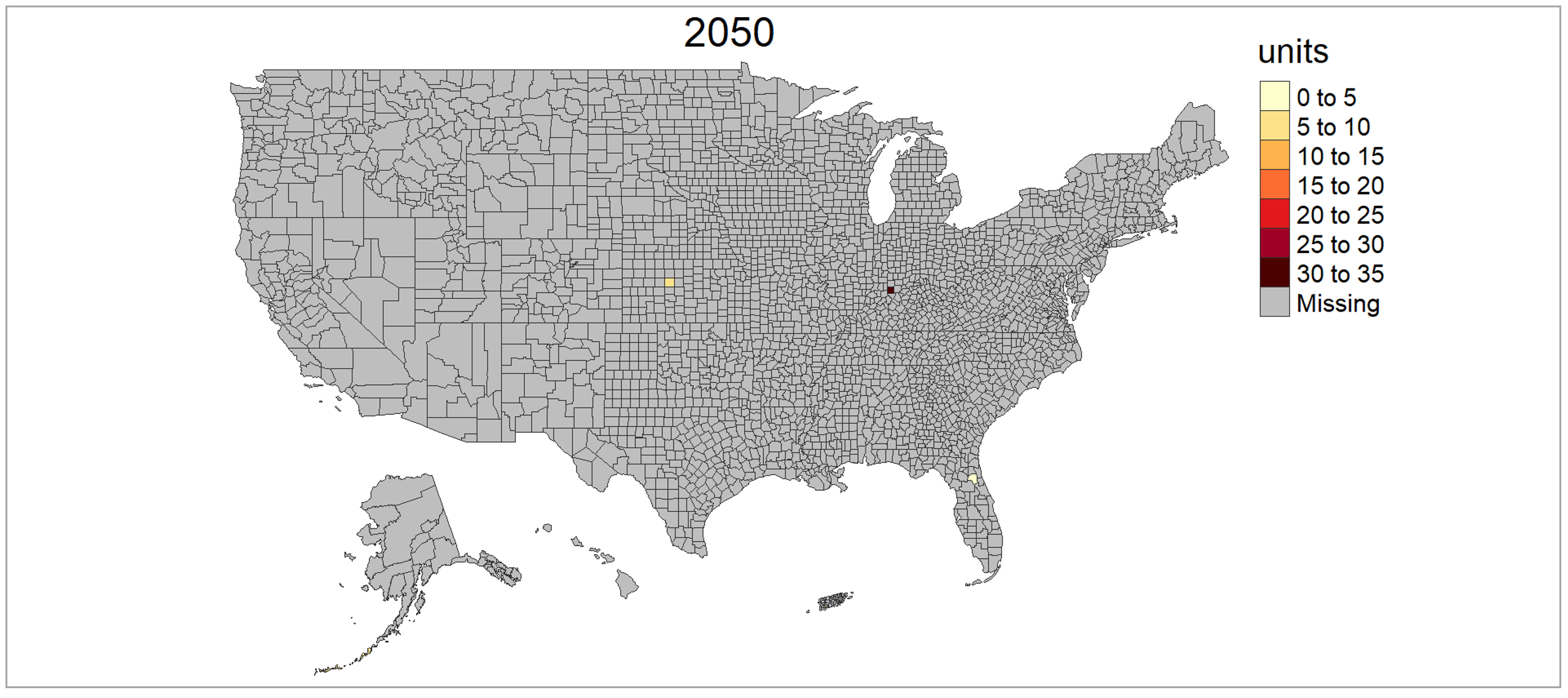
US 49 Counties

library(metis)

unique(mapUS49County@data$subRegion) # Check subRegion Names
unique(mapUS49County@data$subRegionAlt) # Check Alternate names
data = data.frame(subRegion=c("Pender_NC","Larue_KY","Jim Wells_TX","Orange_IN","Putnam_FL","Ellis_KS"),
                  x=c(2050,2050,2050,2050,2050,2050),
                  value=c(5,10,15,34,2,7))
metis.mapsProcess(polygonTable=data,
                  folderName = "vignetteMaps",
                  nameAppend = "_Alt",
                  mapTitleOn = F)

US49 Counties

US 52 Counties

library(metis)

unique(mapUS52County@data$subRegion) # Check subRegion Names
unique(mapUS52County@data$subRegionAlt) # Check Alternate names
data = data.frame(subRegion=c("Aleutians West_AK","Sabana Grande_PR","Kalawao_HI","Orange_IN","Putnam_FL","Ellis_KS"),
                  x=c(2050,2050,2050,2050,2050,2050),
                  value=c(5,10,15,34,2,7))
metis.mapsProcess(polygonTable=data,
                  folderName = "vignetteMaps",
                  nameAppend = "_Alt",
                  mapTitleOn = F)

US52 Counties

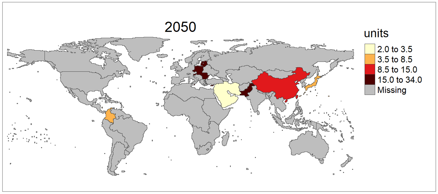
GCAM 32 Regions

library(metis)

unique(mapGCAMBasins@data$subRegion) # Check Available Regions
data = data.frame(subRegion=c("Colombia","China","EU-12","Pakistan","Middle East","Japan"),
                  x=c(2050,2050,2050,2050,2050,2050),
                  value=c(5,10,15,34,2,7))
metis.mapsProcess(polygonTable=data,
                  folderName = "vignetteMaps",
                  mapTitleOn = F)

GCAM 32 Regions

GCAM Basins

library(metis)

unique(mapGCAMBasins@data$subRegion) # Check Available Regions
data = data.frame(subRegion=c("Negro","La_plata","Great","New_England","Indus","Zambezi"),
                  x=c(2050,2050,2050,2050,2050,2050),
                  value=c(5,10,15,34,2,7))
metis.mapsProcess(polygonTable=data,
                  folderName = "vignetteMaps",
                  mapTitleOn = F)

GCAM Basins

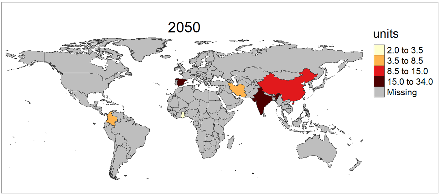
World Countries

library(metis)

unique(mapCountries@data$subRegion) # Check Available Regions
data = data.frame(subRegion=c("Colombia","China","India","Spain","Ghana","Iran"),
                  x=c(2050,2050,2050,2050,2050,2050),
                  value=c(5,10,15,34,2,7))
metis.mapsProcess(polygonTable=data,
                  folderName = "vignetteMaps",
                  mapTitleOn = F)

World Countries

World States

library(metis)

unique(mapStates@data$subRegion) # Check Available Regions
data = data.frame(subRegion=c("Punjab","FL","TX","Faryab","Assam","Lac"),
                  x=c(2050,2050,2050,2050,2050,2050),
                  value=c(5,10,15,34,2,7))
metis.mapsProcess(polygonTable=data,
                  folderName = "vignetteMaps",
                  mapTitleOn = F)

World States

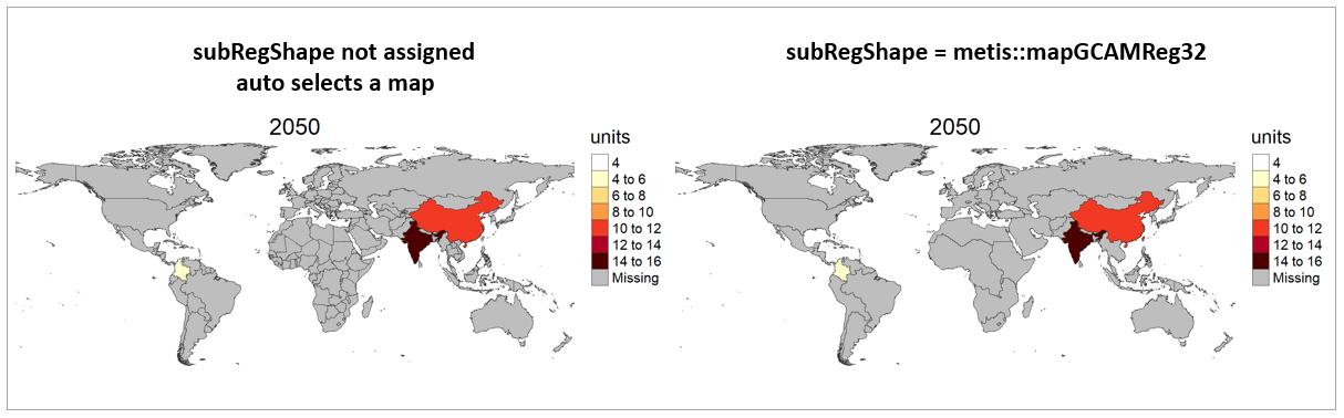
Select Map

Sometimes subRegions can be present on multiple maps. For example “Colombia”, China" and “India” are all members of metis::mapGCAMReg32 as well as metis::mapCountries. If a user knows which map they want to plot their data on they should specify the map in the subRegShape argument.

library(metis)

data = data.frame(subRegion=c("Colombia","China","India"),
                  x=c(2050,2050,2050),
                  value=c(5,10,15))

# Auto selection by metis will choose metis::mapCountries
metis.mapsProcess(polygonTable=data,
                  folderName = "vignetteChooseMap",
                  mapTitleOn = F)

# User can specify that they want to plot this data on metis::mapGCAMReg32
metis.mapsProcess(polygonTable=data,
                  subRegShape = metis::mapGCAMReg32,
                  folderName = "vignetteChooseMap",
                  nameAppend = "Chosen",
                  mapTitleOn = F)

Select Pre-Loaded Map

US 52 Compact

library(metis)

data = data.frame(subRegion=c("AK","HI","PR","MO","TX","WY"),
                  x=c(2050,2050,2050,2050,2050,2050),
                  value=c(5,10,15,34,2,7))
metis.mapsProcess(polygonTable=data,
                  subRegShape=metis::mapUS52Compact,
                  folderName = "vignetteMaps", mapTitleOn = F)

US52Compact

US 52 Counties Compact

library(metis)

unique(mapUS52CountyCompact@data$subRegion) # Check subRegion Names
unique(mapUS52CountyCompact@data$subRegionAlt) # Check Alternate names
data = data.frame(subRegion=c("Aleutians West_AK","Sabana Grande_PR","Kalawao_HI","Orange_IN","Putnam_FL","Ellis_KS"),
                  x=c(2050,2050,2050,2050,2050,2050),
                  value=c(5,10,15,34,2,7))
metis.mapsProcess(polygonTable=data,
                  subRegShape=metis::mapUS52CountyCompact,
                  folderName = "vignetteMaps",
                  nameAppend = "_Alt",
                  mapTitleOn = F)

US52 Counties Compact

Create Custom Map Shape

Users can provide metis.mapsProcess custom shapefiles for their own data if needed. The example below shows how to create a custom shapefile and then plot data on it.

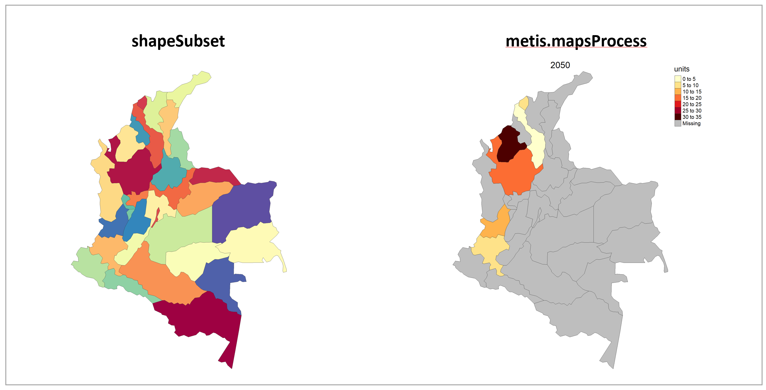
Subset existing shape

library(metis); library(rgdal)

shapeSubset <- metis::mapStates # Read in World States shape file
shapeSubset <- shapeSubset[shapeSubset@data$region %in% c("Colombia"),] # Subset the shapefile to Colombia
shapeSubset@data <- droplevels(shapeSubset@data)
shapeSubset@data <- shapeSubset@data %>% dplyr::rename(states=subRegion) # Lets assume the subRegion column was called "states"
metis.map(shapeSubset,fillCol="states") # View custom shape
head(shapeSubset@data) # review data
unique(shapeSubset@data$states) # Get a list of the unique subRegions

# Plot data on subset
data = data.frame(states=c("Cauca","Valle del Cauca","Antioquia","Córdoba","Bolívar","Atlántico"),
                  x=c(2050,2050,2050,2050,2050,2050),
                  value=c(5,10,15,34,2,7))
metis.mapsProcess(polygonTable=data,
                  subRegShape = shapeSubset,
                  subRegCol = "states",
                  subRegType = "ColombiaStates",
                  folderName = "vignetteMaps_shapeSubset",
                  mapTitleOn = F)

Shape subset

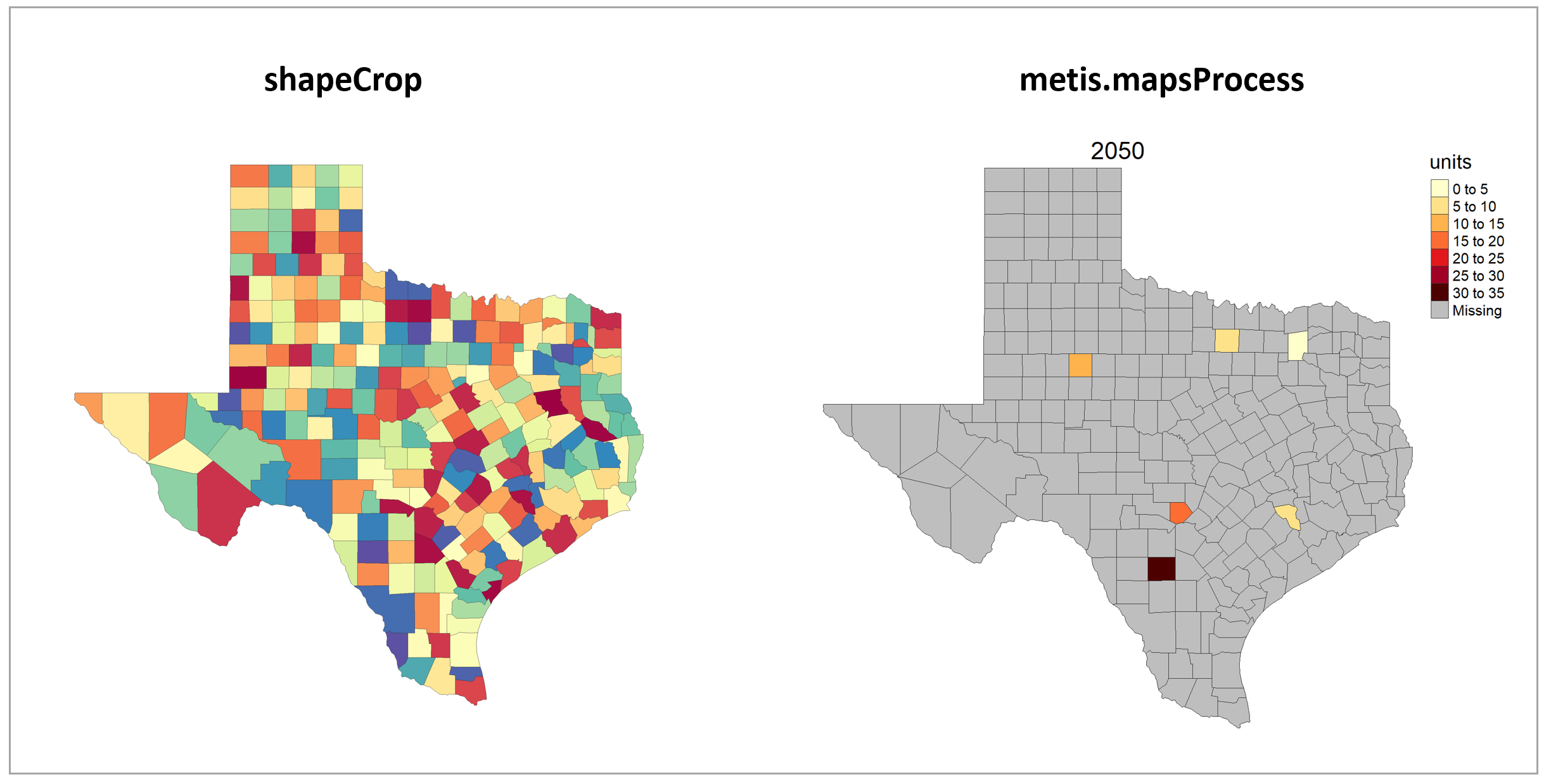
Crop a shape to another shape

For example if someone wants to analyze counties in Texas.

library(metis); library(raster)

shapeSubRegions <- metis::mapUS49County
shapeCropTo <- metis::mapUS49
shapeCropTo <- shapeCropTo[shapeCropTo@data$subRegion %in% c("TX"),]
shapeCropTo@data <- droplevels(shapeCropTo@data)
shapeCrop<- sp::spTransform(shapeCropTo,raster::crs(shapeSubRegions))
shapeCrop <-raster::crop(shapeSubRegions,shapeCropTo)
shapeCrop@data <- shapeCrop@data%>%dplyr::select(subRegion)
shapeCrop$subRegion%>%unique() # Check subRegion names
metis.map(shapeCrop)

# Plot data on subset
data = data.frame(county=c("Wise_TX","Scurry_TX","Kendall_TX","Frio_TX","Hunt_TX","Austin_TX"),
                  x=c(2050,2050,2050,2050,2050,2050),
                  value=c(5,10,15,34,2,7))
metis.mapsProcess(polygonTable=data,
                  subRegShape = shapeCrop,
                  subRegCol = "county",
                  subRegType = "TexasCounties",
                  folderName = "vignetteMaps_shapeCrop",
                  mapTitleOn = F)

Shape Crop

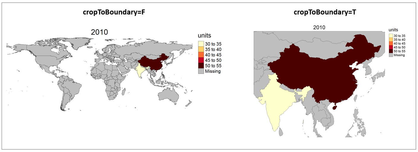
Crop to Boundary

By setting the cropToBoundary argument to T the function will crop your map to the regions with data provided. This is particularly helpful for data plotted on the world maps as shown in the example below:

library(metis)
data = data.frame(subRegion = c("India","China"), year=c(2010,2010),value = c(32,54))
metis.mapsProcess(polygonTable = data, mapTitleOn = F, folderName = "vignetteMaps", cropToBoundary=F, )
metis.mapsProcess(polygonTable = data, mapTitleOn = F, folderName = "vignetteMaps", cropToBoundary=T,
                  nameAppend="Cropped")

Crop to Boundary

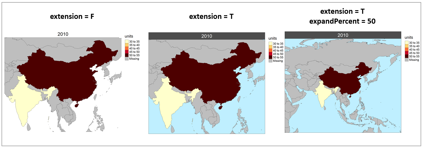
Plot Background

By turning on extension a background layer will be added to any shape map.

library(metis)
data = data.frame(
  subRegion = c("India","China"), year=c(2010,2010), value = c(32,54))
metis.mapsProcess(polygonTable = data, mapTitleOn=F, folderName = "vignetteMaps",
                  cropToBoundary =T,
                  extension = T, nameAppend="Extended")

# Can increase the extnded boundaries by using expandPercent
metis.mapsProcess(polygonTable = data, mapTitleOn=F, folderName = "vignetteMaps",
                  cropToBoundary =T,
                  extension = T, nameAppend="Extended10", expandPercent = 50)

Extended Background

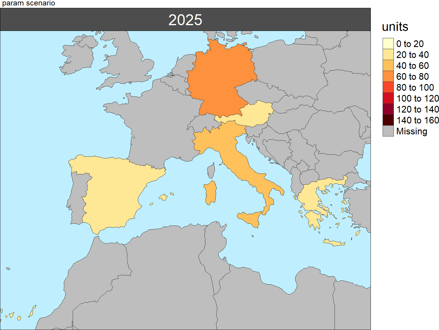
Multi-Year & Animations

library(metis)
data = data.frame(subRegion = c("Austria","Spain", "Italy", "Germany","Greece",
                                "Austria","Spain", "Italy", "Germany","Greece",
                                "Austria","Spain", "Italy", "Germany","Greece",
                                "Austria","Spain", "Italy", "Germany","Greece"),
                  year = c(rep(2025,5),
                               rep(2050,5),
                               rep(2075,5),
                               rep(2100,5)),
                  value = c(32, 38, 54, 63, 24,
                            37, 53, 23, 12, 45,
                            23, 99, 102, 85, 75,
                            12, 76, 150, 64, 90))
metis.mapsProcess(polygonTable = data, folderName ="multiYear",
                  cropToBoundary=T, extension = T )

Multi-year

Multi-year Animation

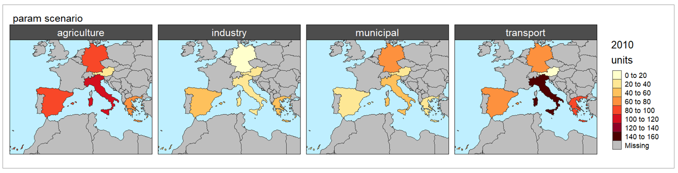
Multi-Class

library(metis)
data = data.frame(subRegion = c("Austria","Spain", "Italy", "Germany","Greece",
                                "Austria","Spain", "Italy", "Germany","Greece",
                                "Austria","Spain", "Italy", "Germany","Greece",
                                "Austria","Spain", "Italy", "Germany","Greece"),
                  class = c(rep("municipal",5),
                               rep("industry",5),
                               rep("agriculture",5),
                               rep("transport",5)),
                  year = rep(2010,20),
                  value = c(32, 38, 54, 63, 24,
                            37, 53, 23, 12, 45,
                            23, 99, 102, 85, 75,
                            12, 76, 150, 64, 90))
metis.mapsProcess(polygonTable = data, folderName ="multiClass",
                  cropToBoundary=T, extension = T )

Multi-class

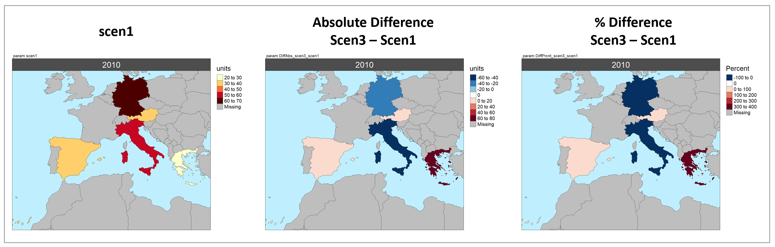
Multi-Scenario Diff plots

With multiple scenarios assigning a scenRef calculates the absolute and percentage difference between the different scenarios and stores them in corresponding folders.

library(metis)
data = data.frame(subRegion = c("Austria","Spain", "Italy", "Germany","Greece",
                                "Austria","Spain", "Italy", "Germany","Greece",
                                "Austria","Spain", "Italy", "Germany","Greece"),
                  scenario = c("scen1","scen1","scen1","scen1","scen1",
                               "scen2","scen2","scen2","scen2","scen2",
                               "scen3","scen3","scen3","scen3","scen3"),
                  year = rep(2010,15),
                  value = c(32, 38, 54, 63, 24,
                            37, 53, 23, 12, 45,
                            40, 44, 12, 30, 99))
metis.mapsProcess(polygonTable = data, folderName ="multiScenario",
                  cropToBoundary=T, extension = T, scenRef="scen1", scenDiff=c("scen3"))

Multi-Scenario Diff

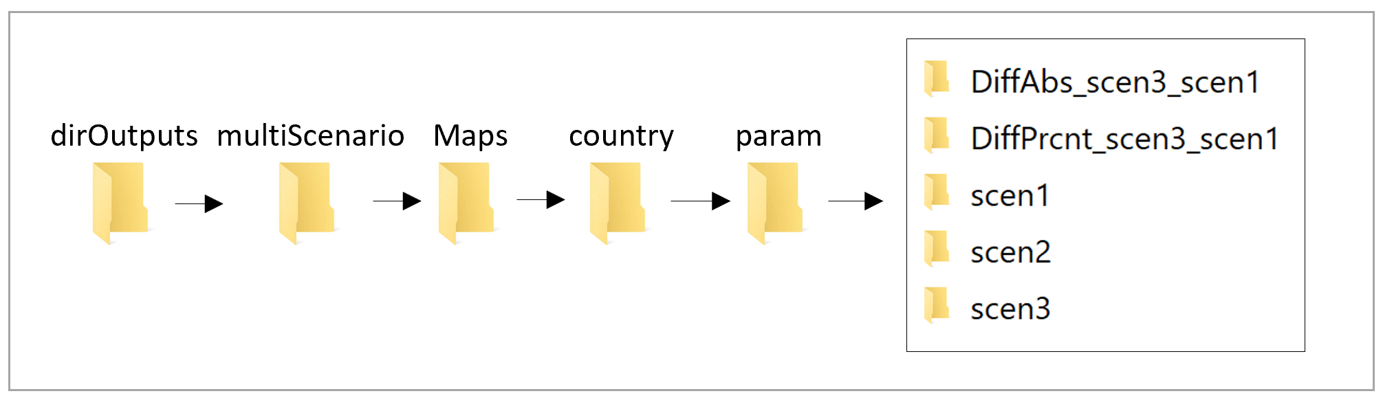
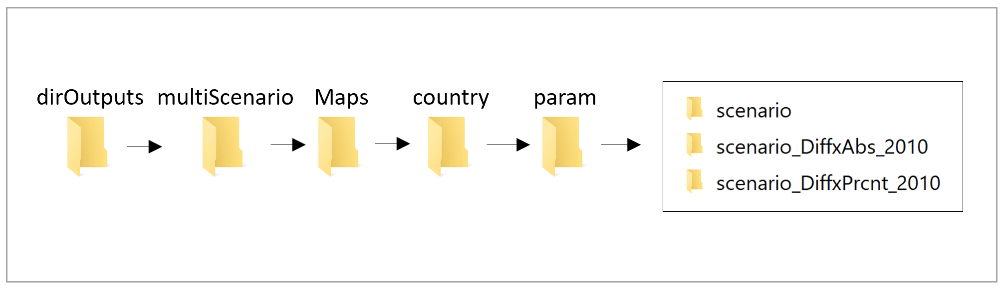
Multi-Scenario Diff Folders

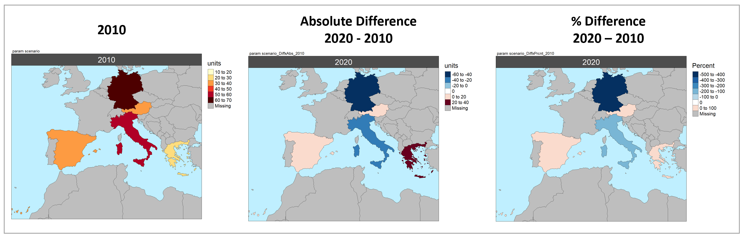
Multi-Year Diff plots

With multiple years assigning a xRef calculates the absolute and percentage difference between the different years and stores them in corresponding folders.

library(metis)
data = data.frame(subRegion = c("Austria","Spain", "Italy", "Germany","Greece",
                                "Austria","Spain", "Italy", "Germany","Greece",
                                "Austria","Spain", "Italy", "Germany","Greece"),
                  year = c(rep(2010,5),rep(2020,5),rep(2030,5)),
                  value = c(32, 38, 54, 63, 24,
                            37, 53, 23, 12, 45,
                            40, 45, 12, 50, 63))
metis.mapsProcess(polygonTable = data, folderName ="multiYear",
                  cropToBoundary=T, extension = T, xRef=2010, xDiff = c(2020))

Multi-Year Diff

Multi-Year Diff Folders

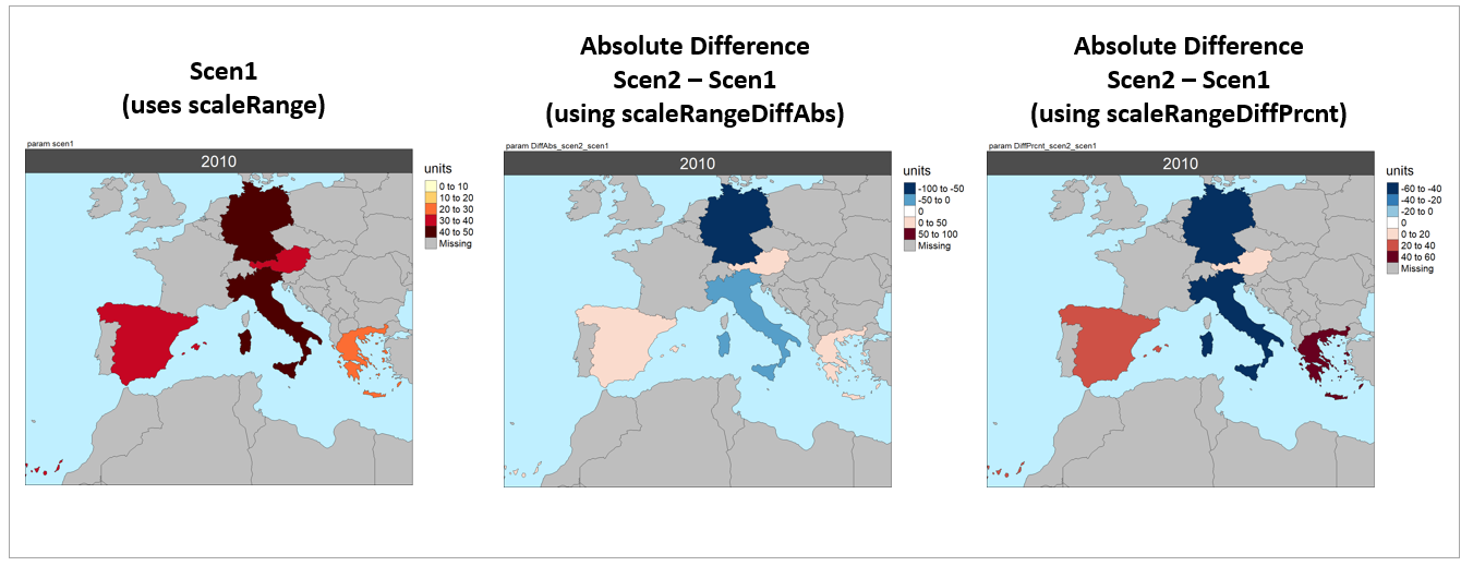
Scale Range

library(metis)
data = data.frame(subRegion = c("Austria","Spain", "Italy", "Germany","Greece",
                                "Austria","Spain", "Italy", "Germany","Greece"),
                  scenario = c("scen1","scen1","scen1","scen1","scen1",
                               "scen2","scen2","scen2","scen2","scen2"),
                  year = rep(2010,10),
                  value = c(32, 38, 54, 63, 24,
                            37, 53, 23, 12, 45))
metis.mapsProcess(polygonTable = data, folderName ="scaleRange",
                  cropToBoundary=T, extension = T, scenRef="scen1",
                  scaleRange = c(0,50), scaleRangeDiffAbs = c(-100,100), scaleRangeDiffPrcnt = c(-60,60))

Scale Range

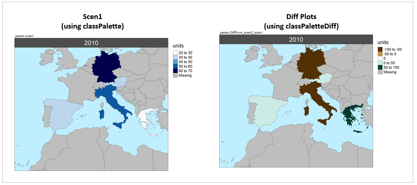
Color Palettes

Can use any R color palette or choose from a list of metis color palettes at colors, maps and params.

library(metis)
data = data.frame(subRegion = c("Austria","Spain", "Italy", "Germany","Greece",
                                "Austria","Spain", "Italy", "Germany","Greece"),
                  scenario = c("scen1","scen1","scen1","scen1","scen1",
                               "scen2","scen2","scen2","scen2","scen2"),
                  year = rep(2010,10),
                  value = c(32, 38, 54, 63, 24,
                            37, 53, 23, 12, 45))
metis.mapsProcess(polygonTable = data, folderName ="colorPalettes",
                  cropToBoundary=T, extension = T, scenRef="scen1",
                  classPalette = "pal_wet", classPaletteDiff = "pal_div_BrGn")

Color Palettes

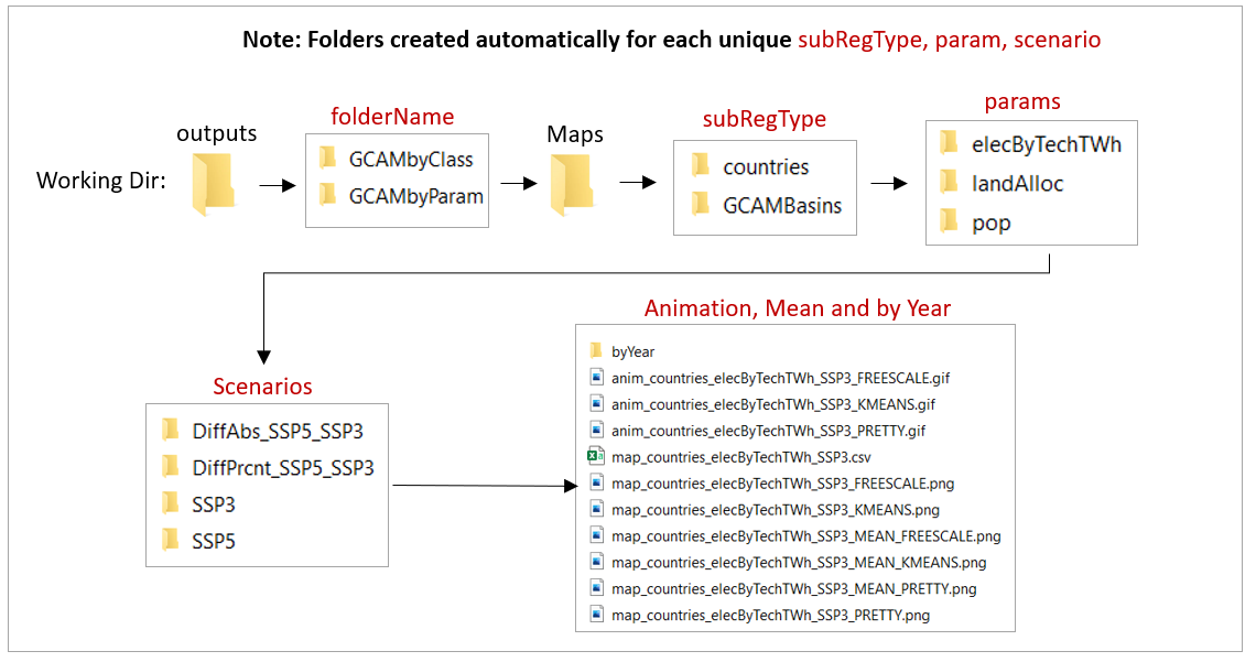
GCAM Results

GCAM results can be read using metis.readgcam to get the data directly into the format ready for mapping. In this example the preloaded GCAM output metis::exampleGCAMproj is used to extract data for chosen parameters from the parameter list. USers can provided a path to their gcam database folder.

Note: The exampleGCAMproj comes with only a few parameters: “elecByTechTWh”,“pop”,“watWithdrawBySec”,“watSupRunoffBasin”,“landAlloc” and “agProdByCrop”

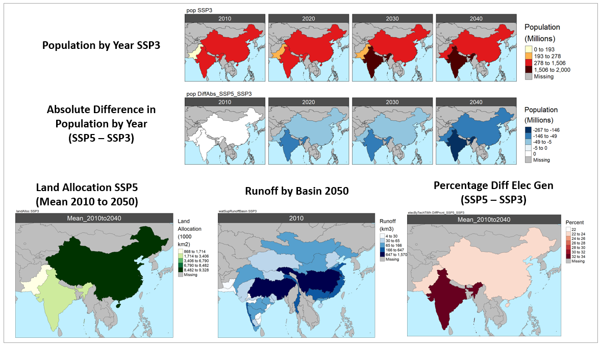
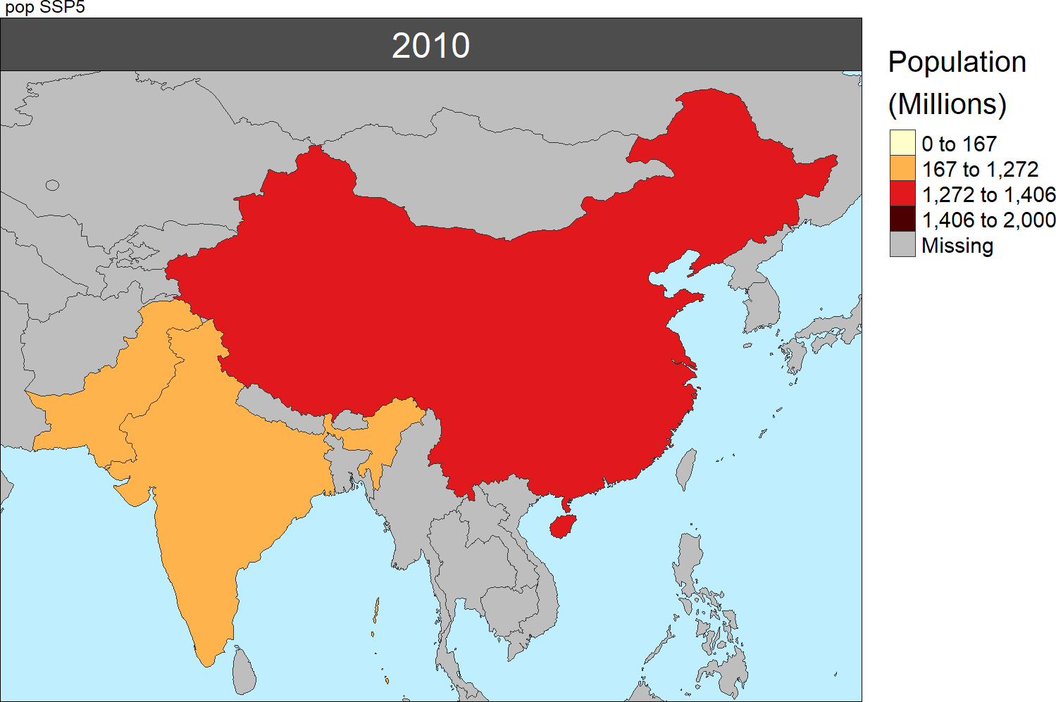
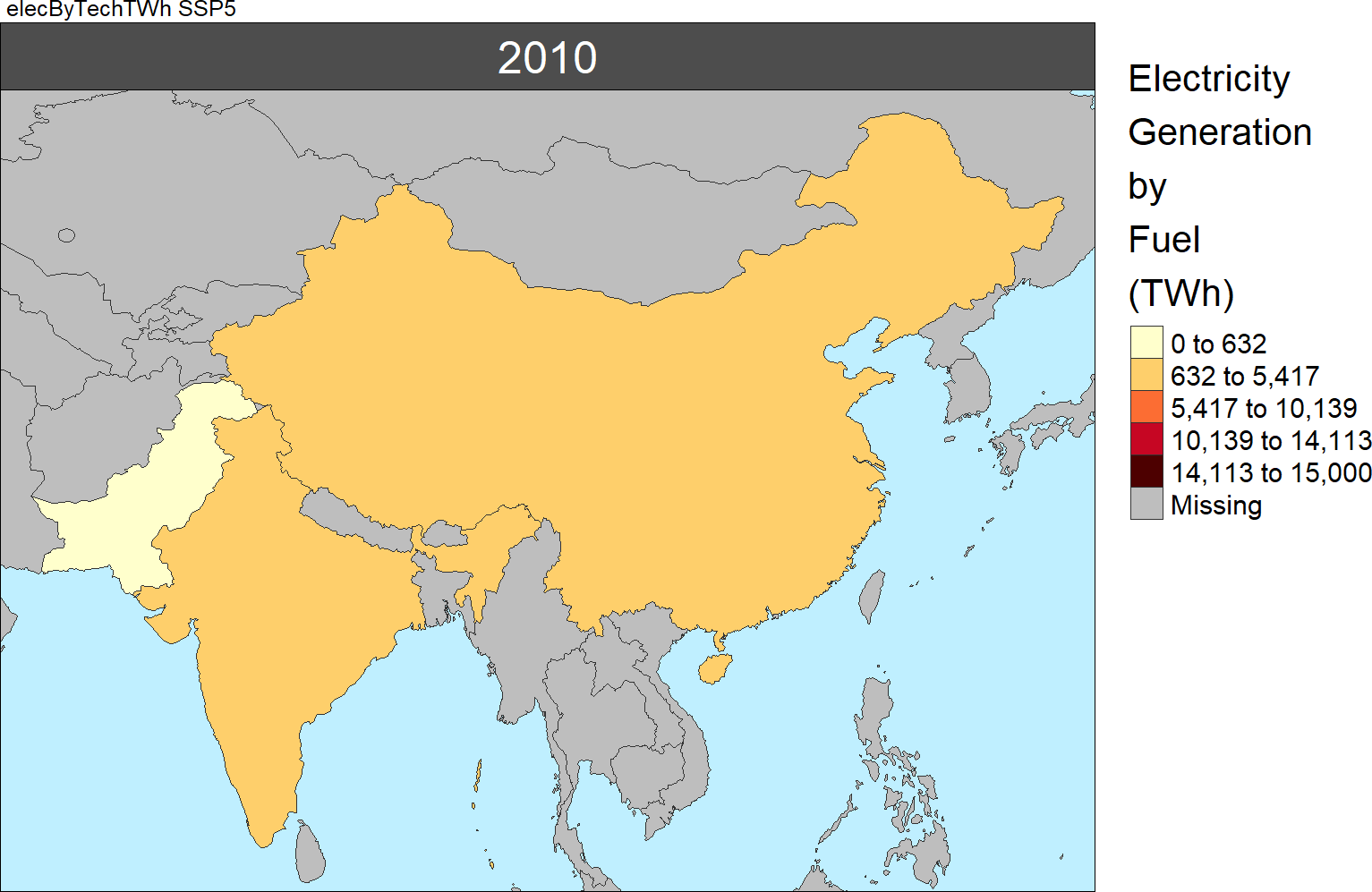
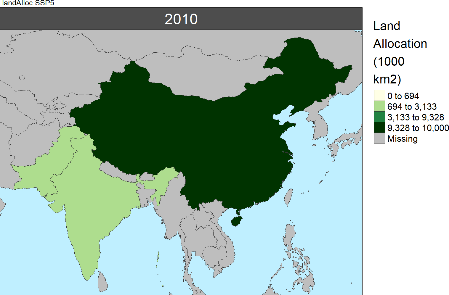
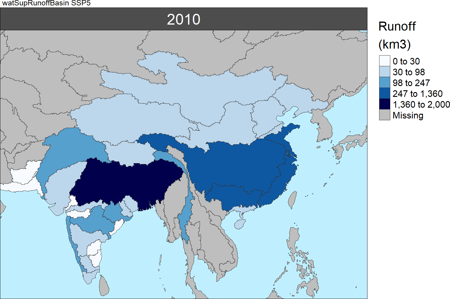
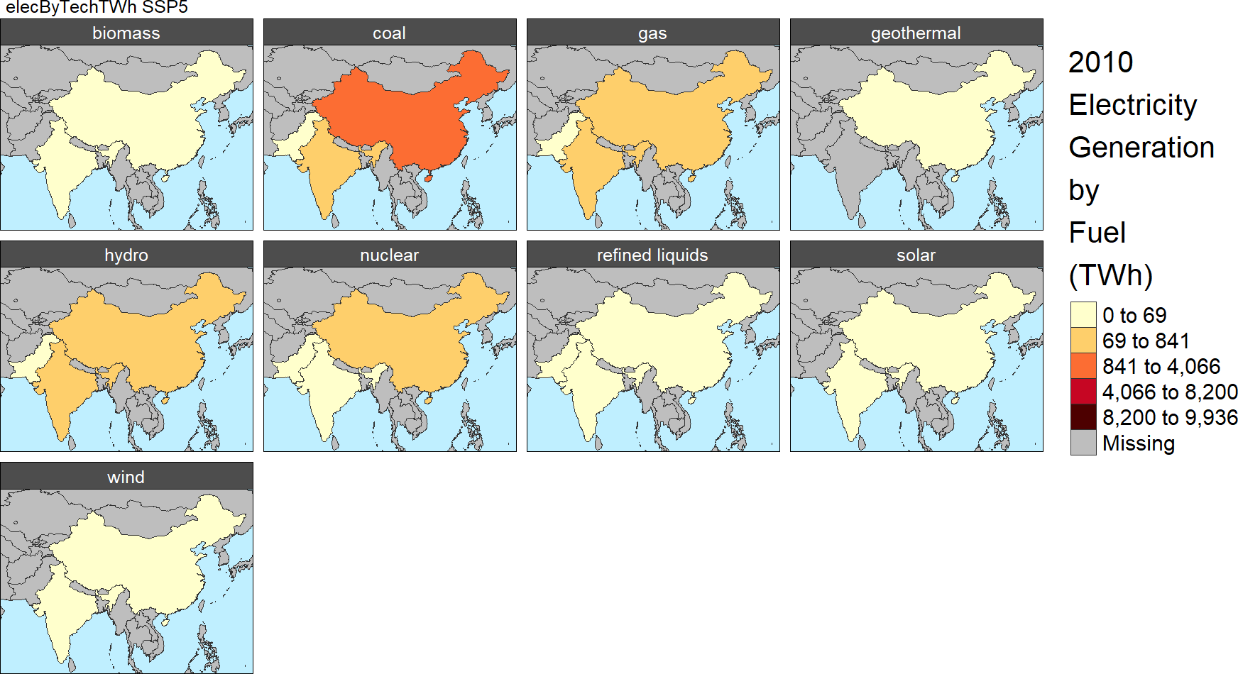
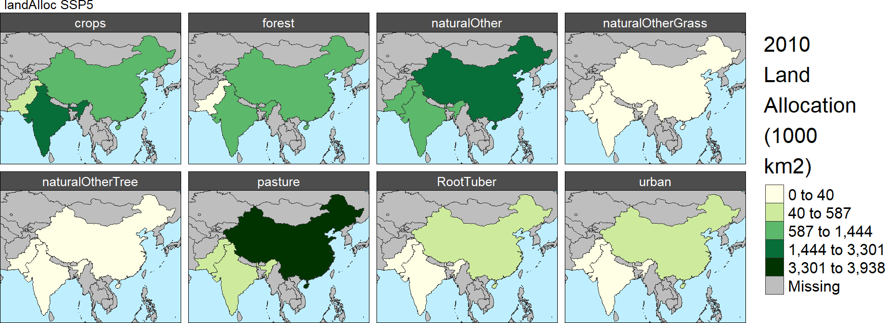
library(metis)

# Read in data from the example Proj file
data <- metis.readgcam (
           #gcamdatabase = “Path_to_GCAMdatabase”,
           dataProjFile = metis::exampleGCAMproj,
           scenOrigNames = c("GCAM_SSP5","GCAM_SSP3"),
           scenNewNames = c("SSP5","SSP3"),
           paramsSelect = c("landAlloc", "elecByTechTWh","watSupRunoffBasin","pop"),  # From Param list ?metis.readgcam
           regionsSelect = c("India","China","Pakistan"))

df <- data$data; df
dfParam <- data$dataAggParam; dfParam
dfClass1 <- data$dataAggClass1; dfClass1
dfClass2 <- data$dataAggClass1; dfClass2

# Plot data aggregated by param
metis.mapsProcess(polygonTable = dfParam, folderName ="GCAMbyParam",
                  cropToBoundary=T, extension = T, xRange = c(2010,2020,2030,2040),
                  scenRef="SSP3", scaleRange = data.frame(param=c("landAlloc", "elecByTechTWh","watSupRunoffBasin","pop"),
                                                          min = c(0,0,0,0),
                                                          max = c(10000,15000,2000,2000)))

# Plot data aggregated by Class1
metis.mapsProcess(polygonTable = dfClass1, folderName ="GCAMbyClass",
                  cropToBoundary=T, extension = T, xRange = c(2010,2020,2030,2040),
                  scenRef="SSP3")

GCAM Outputs Folder Structure

GCAM Maps by Param (Selected)

GCAM Maps by Param Animations (Selected)

Pop	Electricity (TWh)

Land Allocation	Water Withdrawals

GCAM Maps by Class (Selected)

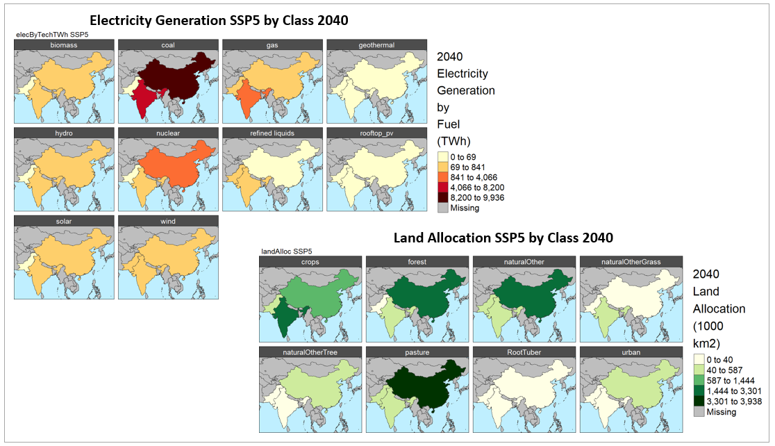
GCAM Maps by Class Animations (Selected)

Electricity (TWh)	Land Allocation