1 Download GCAM SE Asia

Please use the link below to download GCAM.

File	Location
gcamv5p3_seasia	Link

You will need the following prerequisites in order to run GCAM. You will also need at least 8 GB of RAM.

Prerequisite	Link
Java 64	Install Java 64
R	Install R
RStudio	Install RStudio
Windows XML Maker	Install Windows XML Maker

2 Guides

File	Description	Location
gcam_overview.pdf	GCAM overview presentation	Link
gcam_walkthrough.pdf	GCAM walkthrough presentation	Link

3 Scenarios

File	Scenario.Name	Description	Location
configuration_seasia_cities_bau.xml	Ref	Business as Usual Scenario	Link
configuration_seasia_cities_thailand_low.xml	policies_high	Low-ambition sectoral policies in both the MEA area and Rest of Thailand	Link
configuration_seasia_cities_thailand_high.xml	policies_low	High-ambition sectoral policies in both the MEA area and Rest of Thailand	Link

4 Sectoral Policies

The following table lists the policies included in the high and low ambition national policies scenarios. The subsequent sections explain what each of these policies represent and how to adjust them. Each of these policies is implemented using XML add-on file(s) which can be included in the configuration_seasia_cities_thailand_policy.xml file in order to include the policy in the GCAM scenario.

Sector	Policy	Description	High.Ambition	Low.Ambition
Power	RE subsidies	Modify the electricity generation mix by setting generation floors for wind and solar using a subsidy policy	Minimum wind and solar generation correspond with Thailand’s LTS goals	Minimum wind and solar generation correspond with 75% of Thailand’s LTS goals
Power	Coal retirement	Prevent new coal development starting in 2020 and phase out existing coal	Coal is phased out by 2050	Coal is phased out by 2065
Buildings	Building envelope efficiency	Modify the average envelope efficiency of residential and commercial buildings by setting the shell-conductance parameter for each year	Envelope efficiency increases at an annual rate of 4% (residential)/ 4.5% (commercial)	Envelope efficiency increases at an annual rate of 2% (residential)/ 2.5% (commercial)
Buildings	AC efficiency	Modify the average energy efficiency of air conditioners in buildings	Average AC efficiency is 6 W/W by 2030 and 8 W/W by 2050	Average AC efficiency is 4.3 W/W by 2030 and 6 W/W by 2050
Buildings	Lighting efficiency	Phase out non-LED lighting technologies in buildings	Non-LED lighting is phased out by 2030	Non-LED lighting is phased out by 2050
Transportation	EV cost parity	Reduce costs of EVs and hybrid vehicles to reach cost parity with traditional liquids vehicles	EVs reach cost-parity with CEVs by 2030 (passenger)/ 2040 (freight)	EVs reach cost-parity with CEVs by 2050 (passenger)/ 2060 (freight)
Transportation	Liquids phaseout	Phase out combustion engine vehicles	CEVs are phased out by 2050	CEVs are phased out by 2065
Industry	Industrial energy efficiency	Increase average energy efficiency across industrial processes	Industrial energy efficiency increases 1% annually	Industrial energy efficiency increases 0.5% annually
Industry	Industrial hydrogen use	Increase the use of hydrogen in industrial processes	Hydrogen industrial technologies are phased in relatively quickly	Hydrogen industrial technologies are phased in relatively more slowly

For each of the above policies, we are modeling a low-ambition and high-ambition version. For details on the differences between these

4.1 RE Subsidies

Scenario	Files Used	Description
High	wind_solar_floors_high.xml	Sets floors for wind and solar generation corresponding with Thailand’s updated LTS generation goals
Low	wind_solar_floors_low.xml	Sets floors for wind and solar generation corresponding with 75% Thailand’s updated LTS generation goals
Both	wind_solar_input_subsidies.xml	Applies subsidies to relevant wind and solar technologies in order to meet the specified floors

Goal

The goal of this example is to set a minimum value (floor) in GCAM for the amount of electricity generation from wind and solar technologies corresponding with the goals through 2065 presented in the LTS update meeting.

Approach

One way to set a generation floor for each fuel type in GCAM is to use a subsidy policy. This effectively lowers the cost of the relevant electricity generation technologies until the floor is reached.

Background - Policy portfolio standards

A policy-portfolio-standard in GCAM is a policy that can be used to implement taxes, subsidies, floors, ceilings, and constraints. Taxes and subsidies can be specified when the exact amount to be added or subtracted to the price is known. However, a policy-portfolio-standard can also contain a constraint, which acts as either a floor or ceiling for the technology or technologies included. Exact constraints can also be implemented. See the GCAM Policy Examples documentation for more information on how to implement these options.

GCAM Implementation

Create a folder in the input directory eg. ./gcam-core/input/addons.
Download the desired constraint file (either wind_solar_floors_high.xml or wind_solar_floors_low.xml) as well as the subsidy link file wind_solar_input_subsidies to the folder.
To make custom adjustments, optionally change the following within each policy-portfolio-standard tag in the XML:

constraint for each year in which a floor is desired
Set min-price to a large negative value for years in which an exact constraint, rather than a floor, is desired

Within each supplysector tag in the XML, make sure that the corresponding input-subsidy is added within each relevant period for each stub-technology you wish to constrain. Remove each stub-technology that you do not wish to include in the constraint.
Save the xml and then point to it in your configuration file by adding the lines (replace high with low as needed):
<Value name = "scen">../input/addons/wind_solar_floors_high.xml</Value> <Value name = "scen">../input/addons/wind_solar_input_subsidies.xml</Value>

4.2 Coal Phaseout

Scenario	Files Used	Description
Both	no_new_coal.xml	Prevents additional coal capacity from being built starting in 2020
High	coal_shutdown_high.xml	Retires existing coal capacity quickly; all coal is retired by 2050
Low	coal_shutdown_low.xml	Retires existing coal capacity more slowly; all coal is retired by 2065

Goal

The goal of this example is to phase out coal from Thailand’s electricity generation capacity. The difference between the high and low scenarios is how quickly coal is phased out and the year in which the phase-out is completed.

Approach

There are two steps to phase out coal generation. The first is to prevent any new coal capacity from being built; we do this by setting coal shareweights to 0 in all future years. The second step is to gradually retire all existing coal capacity; we do this by shortening coal technologies’ lifetimes and by assigning a shutdown curve to each technology.

Background - Share weights

Share weights are assigned to different subsectors and technology choices in GCAM to represent non-cost factors of consumer choice. They are used primarily to calibrate market shares to historical data but can also be modified to reflect factors such as infrastructure development or shifting societal preferences. For more information on share weights and how they are used in GCAM’s economic choice functions, see the GCAM economic choice documentation. Share weights should not be used to represent cost-related policies. Additionally, shareweight interpolation rules (fixed, linear, or s-curve) can be used to automatically interpolate shareweights between given years.

Background - Energy Technology Retirement

For some energy technologies, such as coal, the “cohort” installed in each period is modeled as a separate technology. Therefore, even if no new capacity is installed in future years, output from the capacity installed in previous years will still be modeled. There are several GCAM parameters that determine the trajectory of output from previously installed technology cohorts. The lifetime is the maximum number of years for which the technology cohort can continue producing output; i.e., a technology cohort installed in year t will no longer produce any output in the year t + lifetime. The s-curve-shutdown-decider is a function that controls the speed at which the technology cohort retires, or reduces its output, within its lifetime. This function depends on a steepness parameter that determines the shape of the function as well as a half-life parameter that sets the number of years after which half of the technology cohort is retired. For more information on retirement parameters, see the GCAM Energy Technologies documentation.

GCAM Implementation

Create a folder in the input directory eg. ./gcam-core/input/addons.
Download the coal shareweight file no_new_coal.xml as well as the desired coal retirement file (either coal_shutdown_high.xml or coal_shutdown_low.xml) to the folder.
To make custom adjustments to the coal retirement trajectory, optionally change the following within each stub-technology tag in the retirement XML:

Use lifetime to adjust the year in which the coal phase-out is complete; the phase-out will be complete x years after 2015, where x is the lifetime.
Use the steepness and half-life within the s-curve-shutdown-decider to adjust the phaseout trajectory; a smaller half-life and larger steepness will result in a faster phase-out.

Save the xmls and then point to them in your configuration file by adding the lines (replace high with low as needed):
<Value name = "scen">../input/addons/no_new_coal.xml</Value> <Value name = "scen">../input/addons/coal_shutdown_high.xml</Value>

4.3 Building Envelope Efficiency

Scenario	Files Used	Description
High	shell_eff_high.xml	Decreases shell conductance from 3.75 in 2020 to 0.487 (residential)/ 0.375 (commercial) in 2070 at an annual rate of 4% (residential)/ 4.5% (commercial)
Low	shell_eff_low.xml	Decreases shell conductance from 3.75 in 2020 to 1.366 (residential)/ 1.057 (commercial) in 2070 at an annual rate of 2% (residential)/ 2.5% (commercial)

Goal

The goal of this example is to represent increasing compliance with the envelope efficiency component of building energy codes. The difference between the low and high scenario versions of this policy is the rate of increase.

Approach

We can use GCAM’s shell-conductance parameter to represent an increase in the average building envelope efficiency according to building energy codes.

Background - Cooling Demand

Cooling demand in GCAM depends on the indoor-outdoor temperature difference (measured using cooling degree days or CDD), the building’s shell conductance, and the building’s external heat gains along with GDP and price factors. For more details and to view the equation used to calculate cooling demand, see the Building service demand section of the GCAM energy demand documentation. GCAM’s shell-conductance parameter is the inverse of building envelope efficiency. Its units are watts per square meter per degree Kelvin and it represents the amount of heat transferred through the building’s exterior when there is a difference between the indoor and outdoor temperature.

GCAM Implementation

Create a folder in the input directory: ./gcam-core/input/addons.
Download the desired xml file (either shell_eff_high.xml or shell_eff_low.xml) to the folder.
To make custom adjustments: within each gcam-consumer tag in the XML, specify the desired shell-conductance values for each year.
Save the xml and then point to it in your configuration file by adding the line (replace high with low as needed):
<Value name = "scen">../input/addons/thailand/shell_eff_high.xml</Value>

4.4 AC Efficiency

Scenario	Files Used	Description
High	ac_eff_high.xml	Increases acerage efficiency of high-efficiency ACs from 3.1 W/W in 2020 to 6 W/W in 2030 and 8 W/W in 2050
Low	ac_eff_low.xml	Increases acerage efficiency of high-efficiency ACs from 3.1 W/W in 2020 to 4.3 W/W in 2030 and 6 W/W in 2050

Goal

The goal of this example is to represent increasing use of the higher and highest efficiency ACs in buildings. The difference between the low and high scenario versions of this policy is the rate of increase of the average AC efficiency.

Approach

We can use GCAM’s efficiency parameter corresponding with the relevant AC technologies to represent an increase in the average AC effiency.

GCAM Implementation

Create a folder in the input directory: ./gcam-core/input/addons.
Download the desired xml file (either ac_eff_high.xml or ac_eff_low.xml) to the folder.
To make custom adjustments: within each period, adjust the efficiency value.
Save the xml and then point to it in your configuration file by adding the line (replace high with low as needed):
<Value name = "scen">../input/addons/thailand/ac_eff_high.xml</Value>

4.5 Lighting Efficiency

Scenario	Files Used	Description
High	buildings_led_high.xml	Gradually phases non-LED residential lighting technology out of the market by 2030
Low	buildings_led_low.xml	Gradually phases non-LED residential lighting technology out of the market by 2050

Goal

The goal of this policy is to represent increasing use of LED lighting in residential buildings and the decreasing use of other, less energy efficient lighting technologies. The difference between the low and high scenario versions of this policy is the year in which 100% LED residential lighting is achieved.

Approach

We can gradually decrease the shareweights of all non-LED residential lighting technologies in order to phase them out of the market. The year in which the non-LED shareweights reach 0 corresponds with the year in which 100% LED residential lighting is achieved.

Background - Share weights

GCAM Implementation

Create a folder in the input directory: ./gcam-core/input/addons.
Download the desired xml file (either buildings_led_high.xml or buildings_led_low.xml) to the folder.
To adjust the year in which 100% LED lighting is achieved: within each non-LED stub-technology tag in the XML, change the to-year in the first interpolation-rule and the from-year in the second. Also change the year of the period tag in which the share-weight is 0.
Save the xml and then point to it in your configuration file by adding the line (replace high with low as needed):
<Value name = "scen">../input/addons/thailand/buildings_led_high.xml</Value>

4.6 EV Cost Parity

Scenario	Files Used	Description
High	ev_cost_parity_high.xml	Reduces EV costs to reach cost parity with liquids vehicles by 2030 (passenger)/ 2040 (freight)
Low	ev_cost_parity_low.xml	Reduces EV costs to reach cost parity with liquids vehicles by 2050 (passenger)/ 2060 (freight)

Goal

The goal of this policy is represent measures to make EVs more competitive with combustion engine vehicles (CEV). The difference between the low and high policies is the year in which EVs reach cost parity with CEVs.

Approach

To represent EV promotion, we use an approach that decreases the cost of EVs relative to CEVs, until the two technologies reach cost parity in some future year. We can do this using GCAM’s input-cost parameter, which represents the non-energy costs of a given technology.

Background - Transportation Cost

In GCAM, the costs of different transportation technologies are comprised of two components: fuel costs and non-fuel costs. A transportation technology’s fuel cost is determined by its vehicle fuel intensity as well as fuel price. The non-fuel costs encompass factors such as capital costs, operation and maintenance, and service costs. These non-fuel costs can be adjusted using the input-cost parameter. For more information on how transportation demand is modeled in GCAM, including cost calculations, see the transportation sections of the GCAM Demand for Energy documentation.

GCAM Implementation

Create a folder in the input directory: ./gcam-core/input/addons.
Download the desired cost parity xml file (either ev_cost_parity_high.xml or ev_cost_parity_low.xml) to the folder.
To make custom adjustments to the EV cost trajectory, set the desired input-cost for each year within eachstub-technology tag in the cost parity xml file.
Save the xml and then point to it in your configuration file by adding the line (replace high with low as needed):

<Value name = "scen">../input/addons/thailand/ev_cost_parity_high.xml</Value>

4.7 CEV phase-out

Scenario	Files Used	Description
High	ldv_liquids_phaseout_high.xml	Phases liquids passenger vehicles out of the market by 2050
Low	ldv_liquids_phaseout_low.xml	Phases liquids passenger vehicles out of the market by 2065

Goal

The goal of this policy is to phase out combustion engine vehicles (CEV) from the market. The difference between the low and high policies is the year in which CEVs are completely phased out of the market.

Approach

To represent a CEV phase-out, we decrease their shareweights over time. The year in which the shareweights are 0 is the year in which CEVs are completely phased out of the market.

Background - Share weights

GCAM Implementation

Create a folder in the input directory: ./gcam-core/input/addons.
Download the desired CEV phase-out xml file (either ldv_liquids_phaseout_high.xml or ldv_liquids_phaseout_low.xml) to the folder.
To adjust the year in which CEVs are completely phased out: within each stub-technology tag in the XML, change the to-year in the first interpolation-rule and the from-year in the second. Also change the year of the period tag in which the share-weight is 0.
Save the xml and then point to it in your configuration file by adding the line (replace high with low as needed):

<Value name = "scen">../input/addons/thailand/ldv_liquids_phaseout_high.xml</Value>

4.8 Industry Energy Efficiency

Scenario	Files Used	Description
High	industry_aeei_high.xml	Increases overall efficiency of industrial processes by 1% annually through 2070
Low	industry_aeei_low.xml	Increases overall efficiency of industrial processes by 0.5% annually through 2070

Goal

The goal of this policy is to represent measures to increase average efficiency of industrial processes. The difference between the low and high scenarios is the rate at which average industrial energy intensity decreases annually.

Approach

To represent a gradual increase in industrial efficiency, we can use GCAM’s aeei parameter, which controls the autonomous energy efficiency improvement (AEEI) of industrial processes.

GCAM Implementation

Create a folder in the input directory: ./gcam-core/input/addons.
Download the desired industrial aeei xml file (either industry_aeei_high.xml or industry_aeei_low.xml) to the folder.
To adjust the rate of industrial energy efficiency increase, change the value of the aeei tag for each desired year.
Save the xml and then point to it in your configuration file by adding the line (replace high with low as needed):

<Value name = "scen">../input/addons/thailand/industry_aeei_high.xml</Value>

4.9 Industry Hydrogen

Scenario	Files Used	Description
High	industry_h2_high.xml	Phases hydrogen industrial technologies into the market relatively quickly
Low	industry_h2_low.xml	Phases hydrogen industrial technologies into the market relatively more slowly

Goal

The goal of this policy is to represent a phase-in of industrial technologies that use hydrogen as a fuel source. The difference between the high and low scenarios is how quickly these technologies are phased into the market.

Approach

To represent a phase-in of hydrogen technologies, we can gradually increase their shareweights.

Background - Share weights

GCAM Implementation

Create a folder in the input directory: ./gcam-core/input/addons.
Download the desired industrial hydrogen technology shareweight xml file (either industry_h2_high.xml or industry_h2_low.xml) to the folder.
To adjust how quicly hydrogen technologies are phased into the market: within each subsector tag in the XML, change the to-year in the interpolation-rule. Also change the year of the period tag in which the share-weight is 1. Be sure that these years match. An earlier year corresponds to a faster phase-in.
Save the xml and then point to it in your configuration file by adding the line (replace high with low as needed):

<Value name = "scen">../input/addons/thailand/industry_h2_high.xml</Value>

5 Emissions Constraints

Scenario	Files Used	Description
Net-Zero CO2	NetZeroC_thailand_2050	CO2 emissions constraint
Net-Zero CO2	Thailand_luc	GHG link file for land use change emissions
Net-Zero CO2	NetZeroC_ROW_2050	CO2 emissions constraint ROW
Net-Zero CO2	ROW_luc	GHG link file for land use change emissions for ROW

Goal

The aim of this example is to demonstrate how to apply an economy-wide emissions constraint for Thailand in accord with its national goals: net-zero CO2 by 2050.

Approach

In GCAM, an emissions constraint can be accomplished by using a ghgpolicy, which is a special case of policy-portfolio-standard that applies to emissions.

Background

To implement a ghgpolicy in GCAM, users specify the total amount of emissions (CO2 or GHG) in a time period. GCAM will then calculate the price on carbon needed to reach the constraint in each period. GCAM finds the least-cost pathway in terms of technology deployment to satisfy the emissions constraint. An economy-wide constraint can be used by itself, or in combination with additional sectoral policies described above. There are some important considerations: (1) what GHG’s are included in the constraint (only CO2?)?, (2) What is the time period for the constraint (e.g., 2050, 2065)?, and (3) What are the emissions in each period (e.g. will emissions decline linearly to zero?)?, (4) Will land use change emissions be included in the constraint?, and (4) what assumptions are made for emissions in the rest of the world? This latter point is important when considering “carbon leakage,” that is, how restrictions in emissions in one geography may lead to a shift in carbon-intensive activities to other locations. Below, we will describe how to implement a CO2 emissions constraint. See the GCAM Policies documentation for more information.

GCAM Implementation

Create a folder in the input directory: ./gcam-core/input/addons.
Download the emissions constraint xml file(s) for Thailand NetZeroC_thailand_2050 and Thailand_luc), as well as those for the rest of the world (ROW), NetZeroC_ROW_2050 and ROW_luc.
The first file, NetZeroC_thailand_2050.xml, specifies emissions in units of tonnes of carbon (not CO2) in each period. One way to determine the emissions constraint for each period is to examine the CO2 emissions in the reference case (See ModelInterface: “CO2 emissions by region”). Based on the reference emissions, one can create an emissions constraint accordingly, depending on the start date of the emissions constraint, end goal, and steepness of the decrease in emissions. In this case, we want to reach net-zero CO2 emissions in 2050. The example specifies a linear decrease from 2025 to 2050. (A negative number in 2050 is used instead of 0, because this is easier for GCAM to solve). Other emissions constraints can be adopted instead of net-zero CO2 emissions in 2050.
One needs to decide whether and how land use change emissions are incorporated into the constraint. GCAM accounts for fossil fuel and industry CO2 emissions separately from land use change CO2 emissions. The Thailand_luc.xml specifies how land use change CO2 emissions (LUC-CO2) in Thailand are linked to the ghgpolicy (“CO2”). There are two parameters: price-adjust and demand-adjust. Price-adjust is used to convert prices for different GHG’s. A price-adjust of 1.0 for LUC-CO2 means the market price on LUC-CO2 emissions is the same as the price applied to fossil fuel and industry CO2 emissions. A demand-adjust of 1 means that LUC-CO2 emissions are counted in the emissions constraint. These two parameters can be adjusted. In the sample files we have a price-adjust of 1, and a demand-adjust of 1. The same files for the rest of the world (ROW) are included to make sure that the same constraint is applied outside of Thailand in order to prevent carbon leakage.
Save the xml files and then point to them in your configuration file by adding the line:

<Value name = "scen">../input/addons/thailand/NetZeroC_thailand_2050.xml</Value> <Value name = "scen">../input/addons/thailand/Thailand_luc.xml</Value> <Value name = "scen">../input/addons/thailand/NetZeroC_ROW_2050.xml</Value> <Value name = "scen">../input/addons/thailand/ROW_luc.xml</Value>

6 Diagnostics

This section describes how to explore and compare the final output data using GCAM’s post-processing tools.

6.1 Download database

Please use the link below to download the output database from GCAM. This database contains model results for the scenarios described above.

File	Location
database_seasia_cities	Link

6.2 Extract GCAM Data

gcamextractor is an R package used to extract and process GCAM data and manipulate into standardized tables. gcamextractor converts GCAM outputs into commonly used units as well as aggregates across different classes and sectors for easy use in plots, maps and tables. For more information, please reference the documentation page found here.

The first step is to create a path to the GCAM database, found in the output folder of your GCAM folder, and a list of desired parameters. The readgcam() function also requires region names and a specific output folder. Because reading in many parameters can take several minutes, we will be using existing outputs, found in your working directory’s “gcamextractor” folder, generated by the code below.

sample_path <- "./output/database"

sample_params <- "summary"

regions <- c("Bangkok", "SamutPrakan", "Nonthaburi", "Rest of Thailand", "Thailand")

aggregate_regions <- list(c("Bangkok", "SamutPrakan", "Nonthaburi"), regions)

aggregate_region_names <- c("MEA area", "All of Thailand")

data <- gcamextractor::readgcam(gcamdatabase = sample_path,
                                paramsSelect = sample_params,
                                regionsSelect = regions,
                                regionsAggregate = aggregate_regions,
                                regionsAggregateNames = aggregate_region_names,
                                folder = "../data/thailand/gcamextractor")

thailand <- read.csv("../data/Thailand/all_data.csv")

thailand_with_hist <- read.csv("../data/Thailand/all_data_with_hist.csv")

6.3 Plot Figures

rchart is a comprehensive charting package to plot and compare data across scenarios, regions, sectors and time periods in GCAM. The following tabs show initial diagnostics of the sectoral policy scenarios for all of Thailand as well as the MEA area.

6.3.1 Thailand

6.3.1.1 Summary figures

6.3.1.1.1 Socioeconomic summary

socioeconomic_parameters <- c("pop", "gdp", "gdpPerCapita")

socioeconomic <- thailand %>%
  filter(param %in% socioeconomic_parameters,
         region %in% c("MEA area", "Thailand"),
         scenario == scenRef_name) %>%
  mutate(param = units) %>% 
  rchart::chart(save = F, 
                show = F,
                size_text = 19,
                chart_type = "chart_param_absolute")

socioeconomic$chart_param_Thailand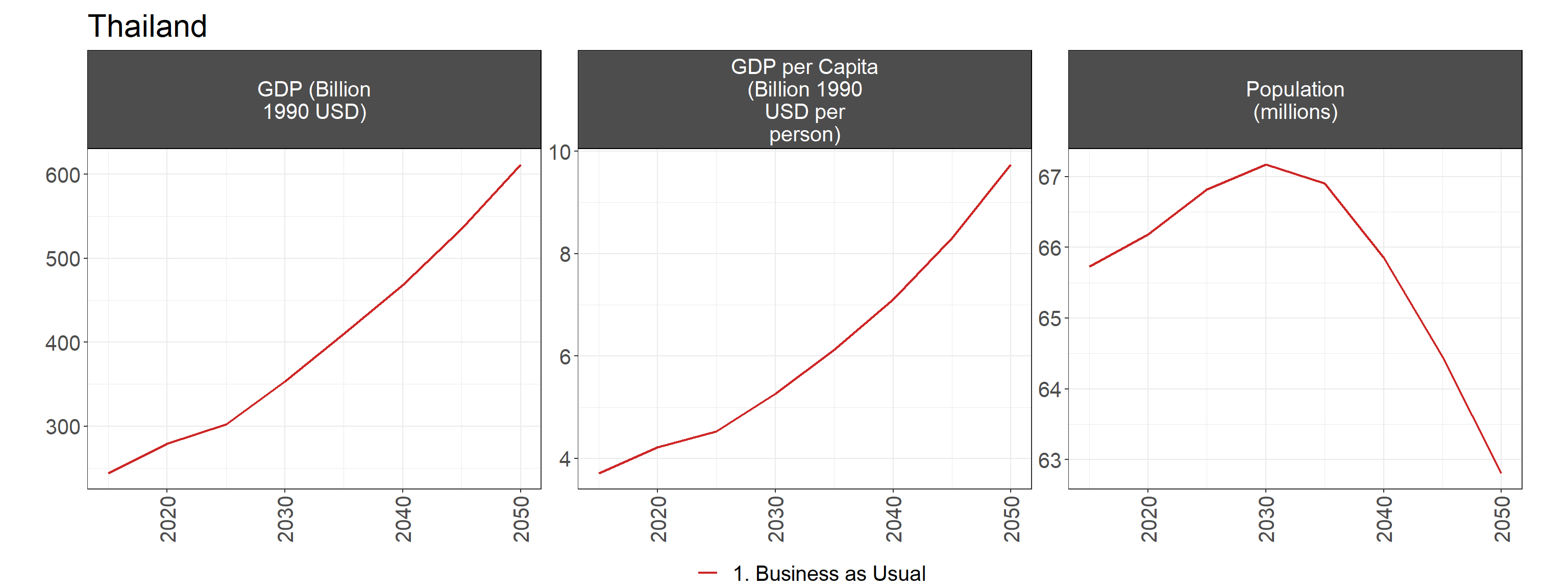

GDP, per capita GDP, and population in Thailand from 2020 to 2065. Only the BAU scenario is shown since socioeconomic assumptions are consistent between scenarios.

6.3.1.1.2 CO2 Emissions by Sector

emissions_line_params <- c("emissCO2BySectorNoBio")

emissions_line <- thailand %>% filter(param %in% emissions_line_params,
                           region %in% c("All of Thailand", "MEA area")) %>%
  mutate(param = units) %>% 
  rchart::chart(chart_type = "param_absolute",
                save = F, 
                show = F,
                size_text = 19)

emissions_line$`chart_param_All of Thailand`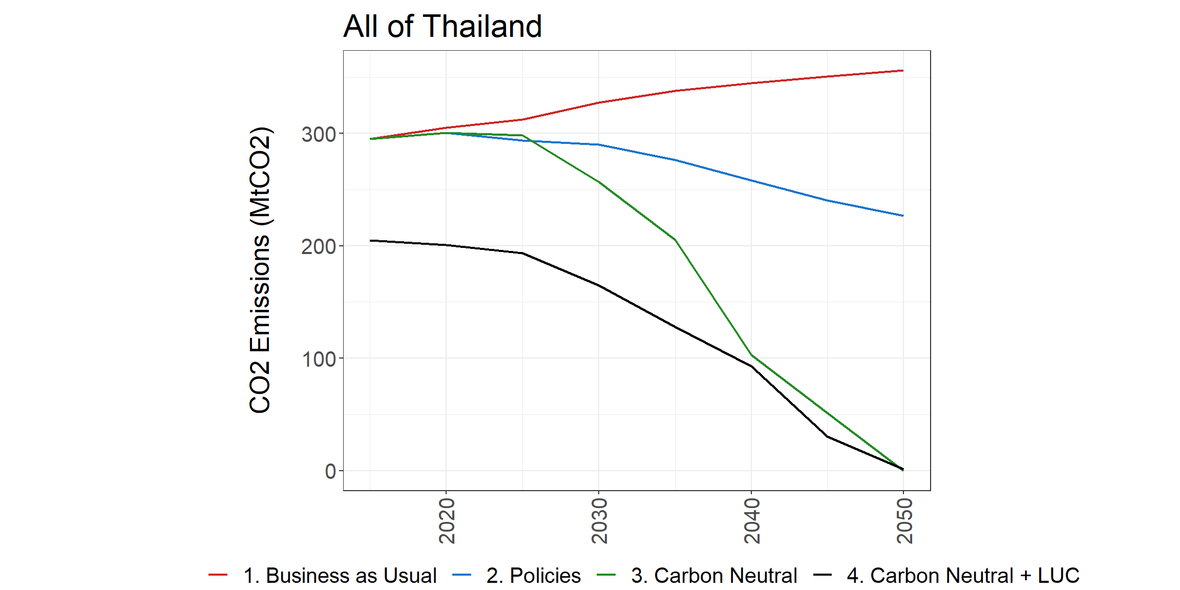

Total national CO2 emissions (left) and GHG emissions (right) in the reference scenario and the low and high policies scenarios

emissions_params <- c("emissCO2BySectorNoBio")

emissions_bar <- thailand %>% filter(param %in% emissions_params,
                                     region %in% c("All of Thailand", "MEA area")) %>%
  filter(class != "LUC") %>% 
  mutate(class = case_when(class %in% c("hydrogen", "refining") ~ "Industry",
                           T ~ class)) %>% 
  group_by(scenario, region, x, class, param, units) %>% 
  summarize(value = sum(value)) %>% 
  ungroup() %>% 
  mutate(param = units) %>% 
  rchart::chart(save = F, 
                show = F,
                size_text = 19,
                scenRef = scenRef_name,
                summary_line = T,
                chart_type = "class_absolute",
                palette = c("BECCS" = "forestgreen"),
                ncol = 4)

emissions_bar$`chart_class_All of Thailand`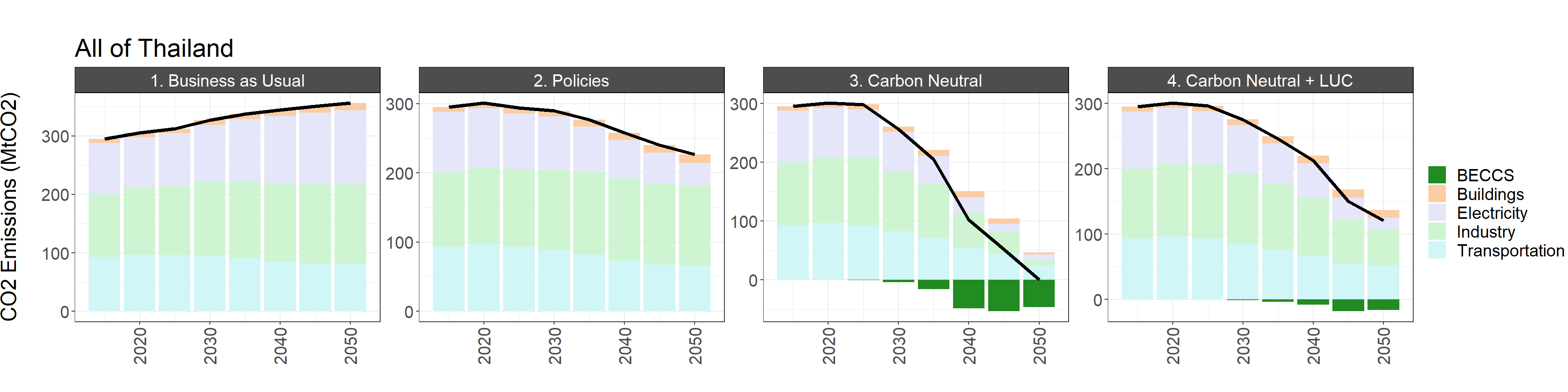

National CO2 emissions by sector, GHG emissions by gas, and GHG emissions by sector in the reference scenario and the low and high policies scenarios

One of rchart’s chart types is class_diff_absolute, which shows the reference (BAU) scenario on the left and the difference between each policy scenario and the reference scenario on the right. For example, the policies_high_diffAbs panels in the chart below show the difference in CO2 and GHG emissions by sector and gas in the policies_high scenario compared to the Ref scenario.

emissions_diff <- thailand %>% filter(param %in% emissions_params,
                                      region %in% c("All of Thailand", "MEA area")) %>%
  filter(class != "LUC") %>% 
  mutate(class = case_when(class %in% c("hydrogen", "refining") ~ "Industry",
                           T ~ class)) %>% 
  group_by(scenario, region, x, class, units) %>% 
  summarize(value = sum(value)) %>% 
  ungroup() %>% 
  mutate(param = units) %>% 
  rchart::chart(save = F, 
                show = F,
                size_text = 19,
                scenRef = scenRef_name,
                summary_line = F,
                chart_type = "class_diff_absolute",
                palette = c("BECCS" = "forestgreen"))

emissions_diff$`chart_class_diff_absolute_All of Thailand`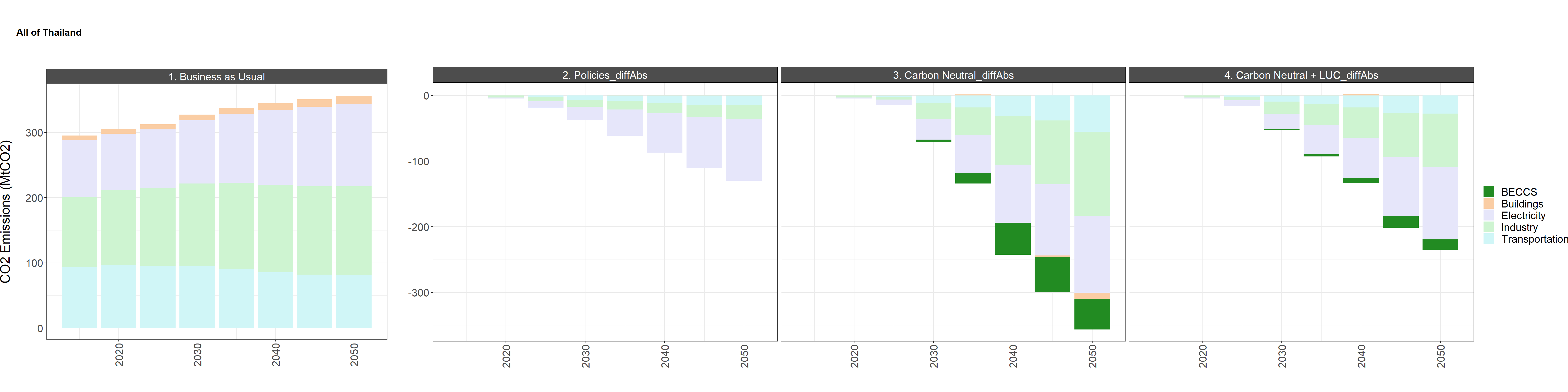

Difference in national CO2 and GHG emissions by sector and gas between the reference scenario (left) and the low and high policy scenarios (right)

6.3.1.1.3 Final Energy by Fuel and Sector

energy_parameters <- c("energyFinalConsumBySecEJNoFeedstock", "energyFinalByFuelEJNoFeedstock")

energy <- thailand %>% 
  filter(param %in% energy_parameters,
         region %in% c("All of Thailand", "MEA area")) %>%
  mutate(param = units) %>%
  rchart::chart(save = F, 
                show = F,
                size_text = 20,
                scenRef = scenRef_name,
                chart_type = c("class_absolute", "class_diff_absolute"),
                scales = "fixed",
                ncol = 4)

energy$`chart_class_All of Thailand`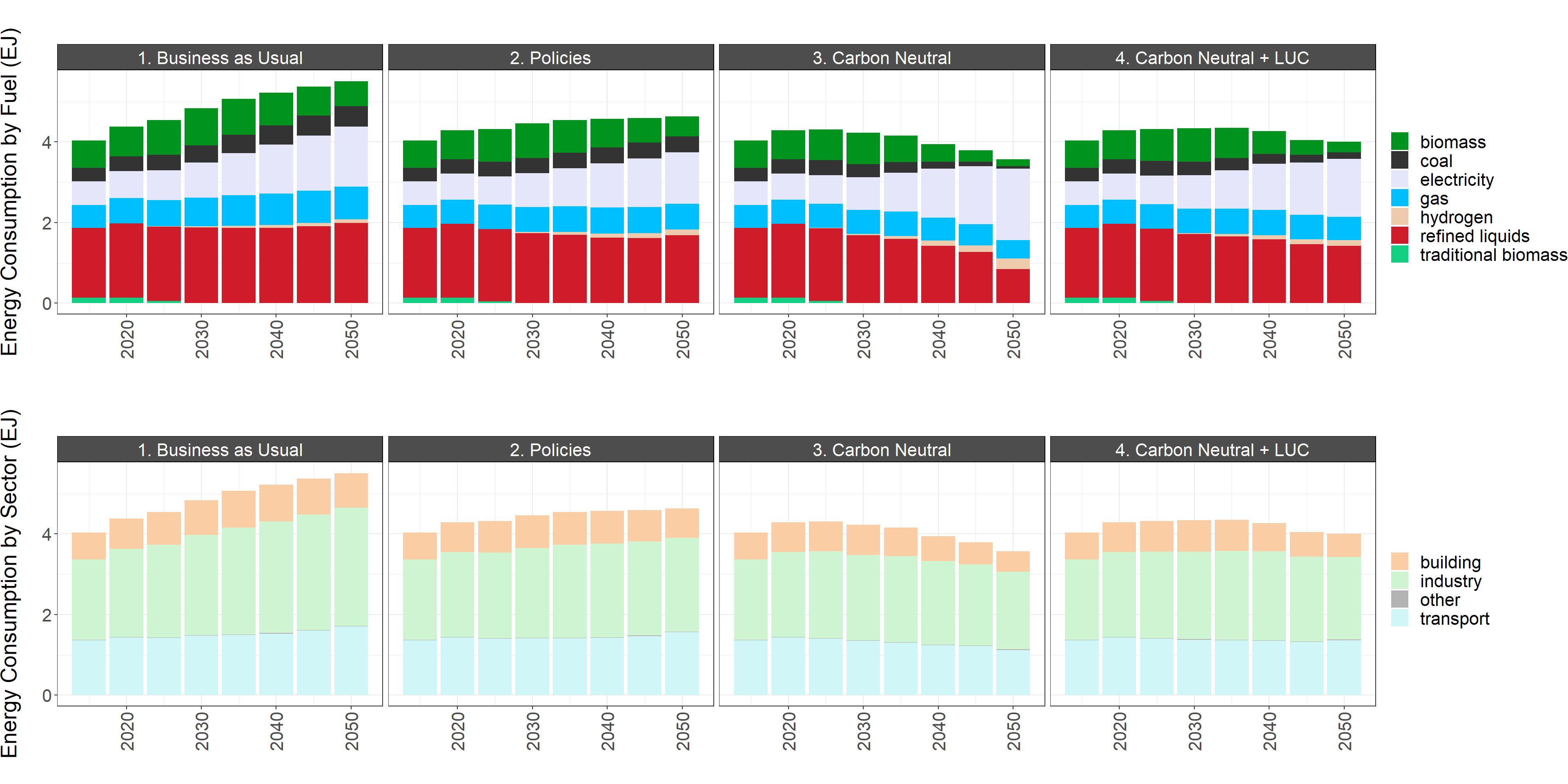

National final energy consumption by fuel and sector in the reference scenario and the low and high policies scenarios

energy$`chart_class_diff_absolute_All of Thailand`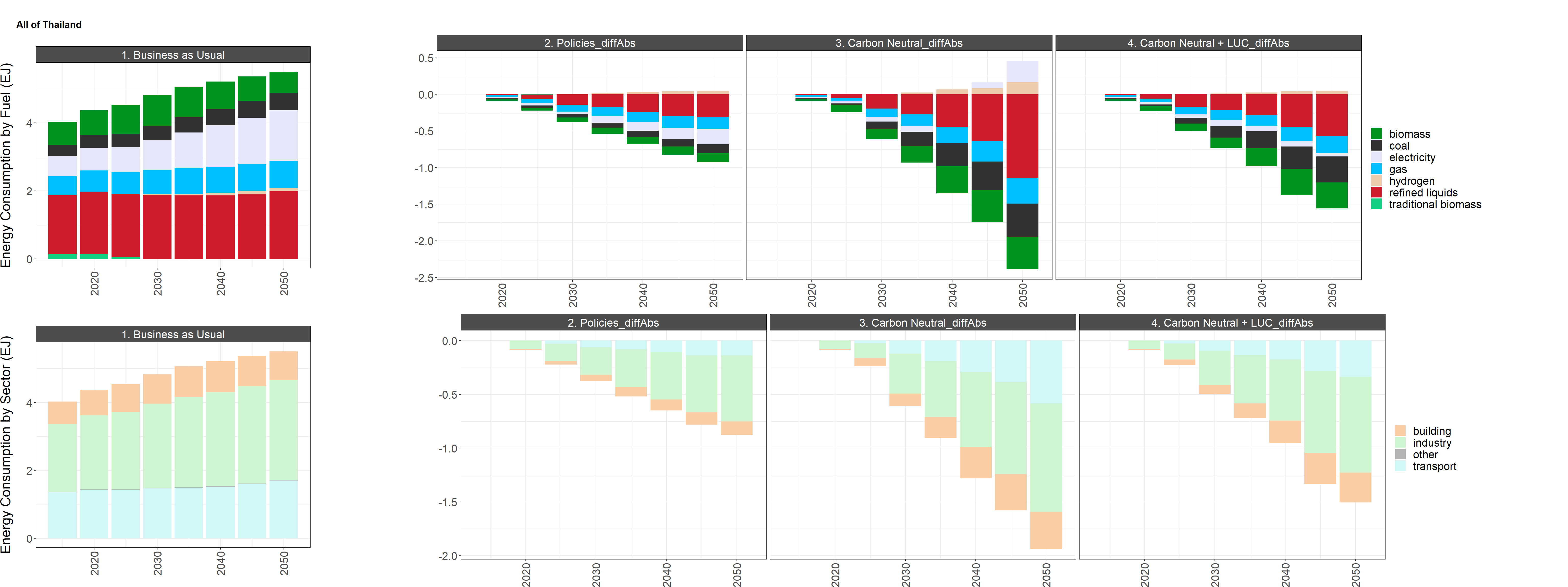

Difference in national final energy consumption by fuel and sector between the reference scenario (left) and the low and high policy scenarios (right)

6.3.1.1.4 Electricity Generation and Consumption

elec_parameters <- c("elecByTechTWh", "elecConsumByDemandSectorTWh")

electricity <- thailand %>% 
  filter(param %in% elec_parameters,
         region %in% c("All of Thailand", "MEA area"),
         !grepl("backup", class)) %>%
  mutate(param = units) %>%
  rchart::chart(save = F, 
                show = F,
                size_text = 19,
                scenRef = scenRef_name,
                chart_type = c("class_absolute", "class_diff_absolute"),
                scales = "fixed",
                ncol = 4)

electricity$`chart_class_All of Thailand`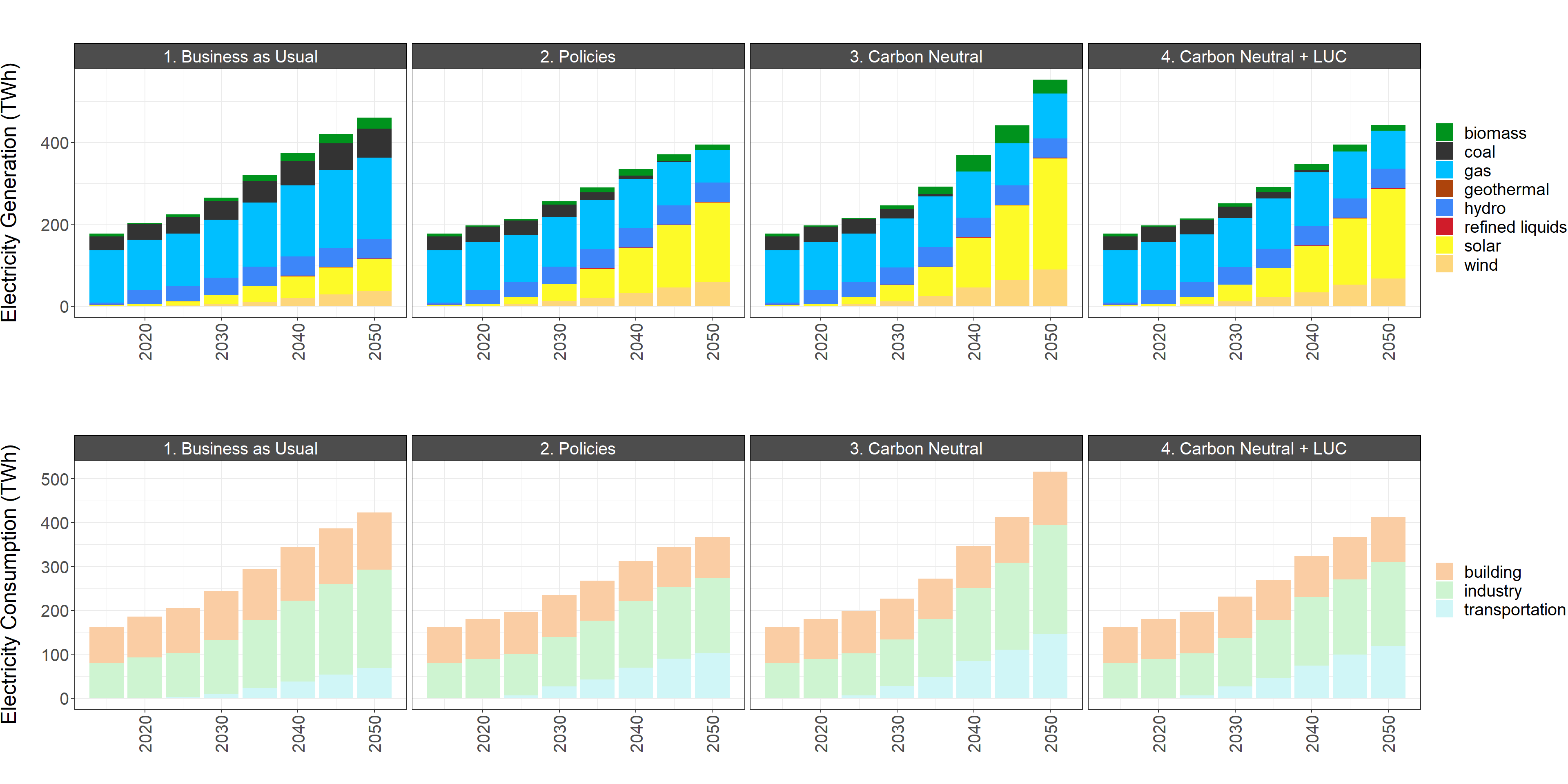

National electricity generation by fuel, electricity consumption by sector, and power sector GHG emissions by gas and fuel in the reference scenario and the low and high policies scenarios

electricity$`chart_class_diff_absolute_All of Thailand`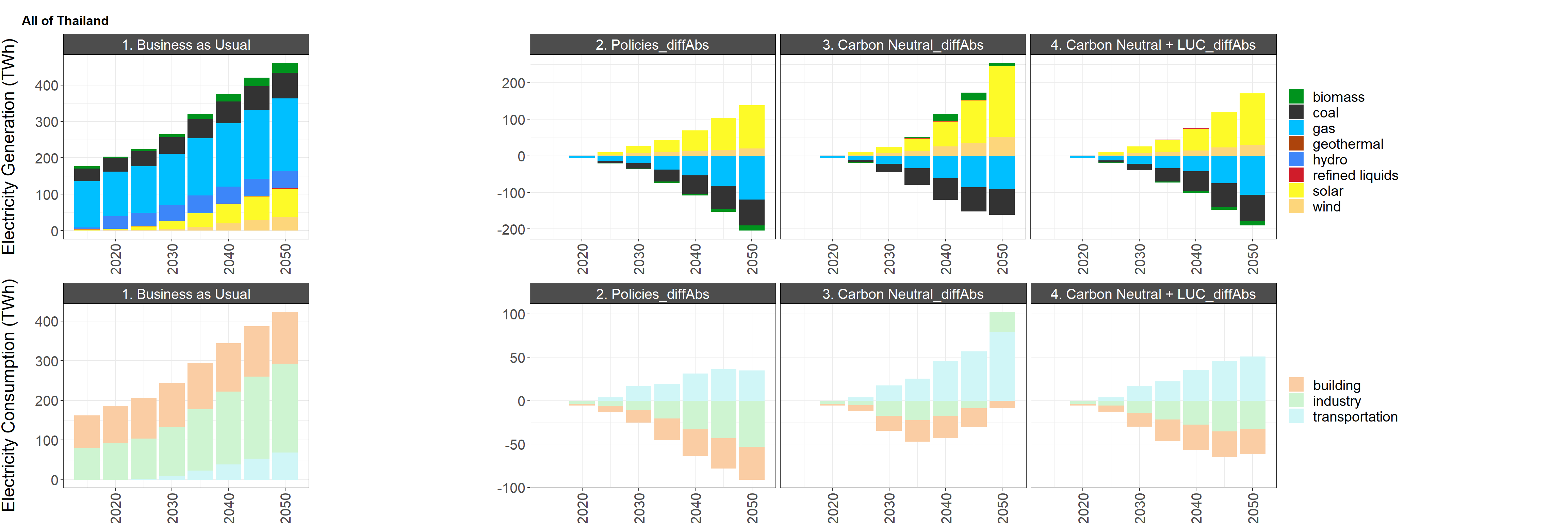

Difference in national electricity generation by fuel, electricity consumption by sector, and power sector GHG emissions by gas and fuel between the reference scenario (left) and the low and high policy scenarios (right)

6.3.1.2 Sectoral details

6.3.1.2.1 Buildings

buildings_params <- c("energyFinalSubsecByFuelBuildEJ", 
                      "energyFinalSubsecBySectorBuildEJ")

building_sector_colors <- c(
  "commercial ACMV" = "#b2e2e2",
  "commercial cooking" = "#66c2a4",
  "commercial lighting" = "#2ca25f",
  "commercial other" = "#006d2c",
  "residential ACMV" = "#fee8c8",
  "residential cooking" = "#fdd49e",
  "residential lighting" = "#fdbb84",
  "residential other" = "#fc8d59")

buildings <- thailand %>% 
  filter(param %in% buildings_params,
         region %in% c("All of Thailand", "MEA area"),
         class != "global solar resource") %>%
  mutate(param = units) %>%
  rchart::chart(save = F, 
                show = F,
                size_text = 19,
                scenRef = scenRef_name,
                palette = building_sector_colors,
                chart_type = c("class_absolute", "class_diff_absolute"),
                scales = "fixed",
                ncol = 4)

buildings$`chart_class_All of Thailand`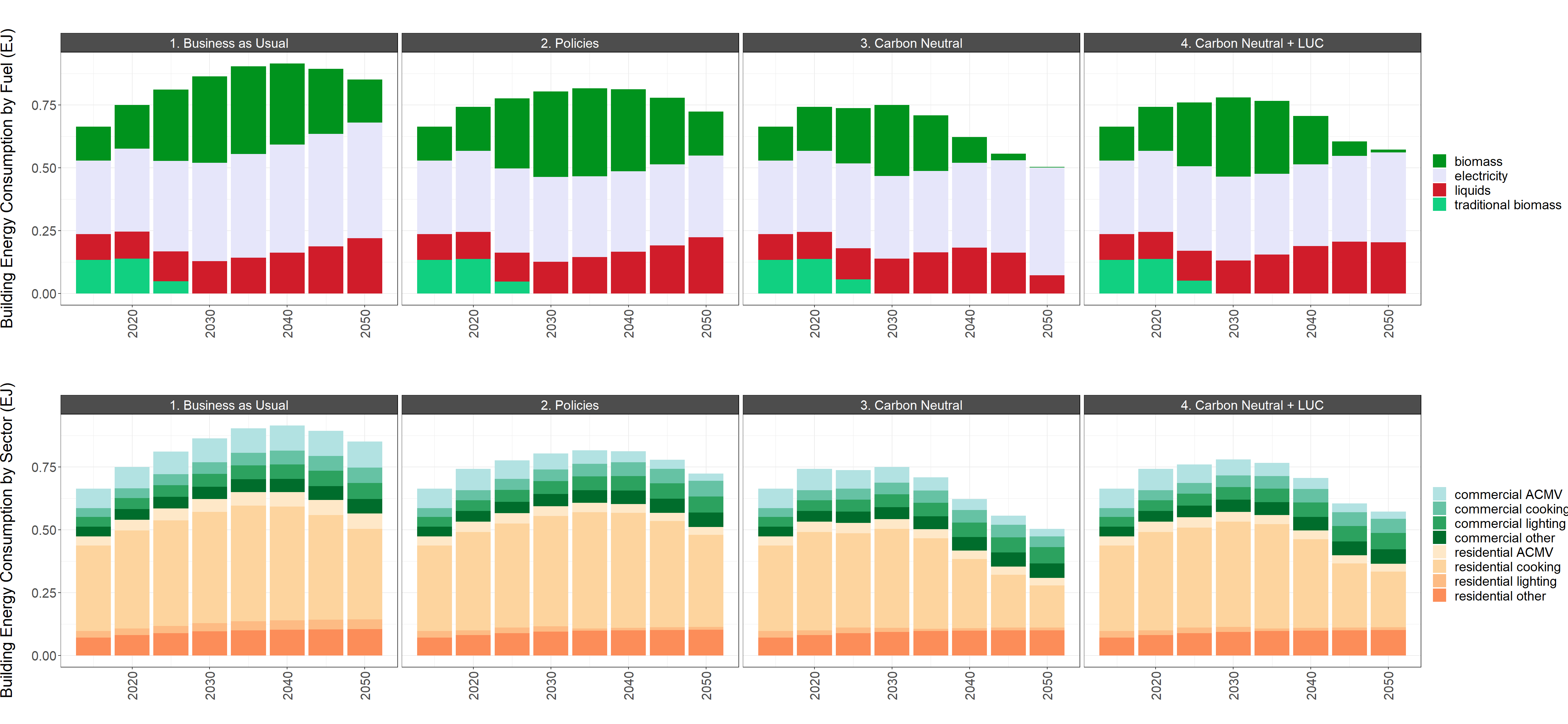

National buildings sector final energy by fuel and by service in the reference scenario and the low and high policies scenarios

buildings$`chart_class_diff_absolute_All of Thailand`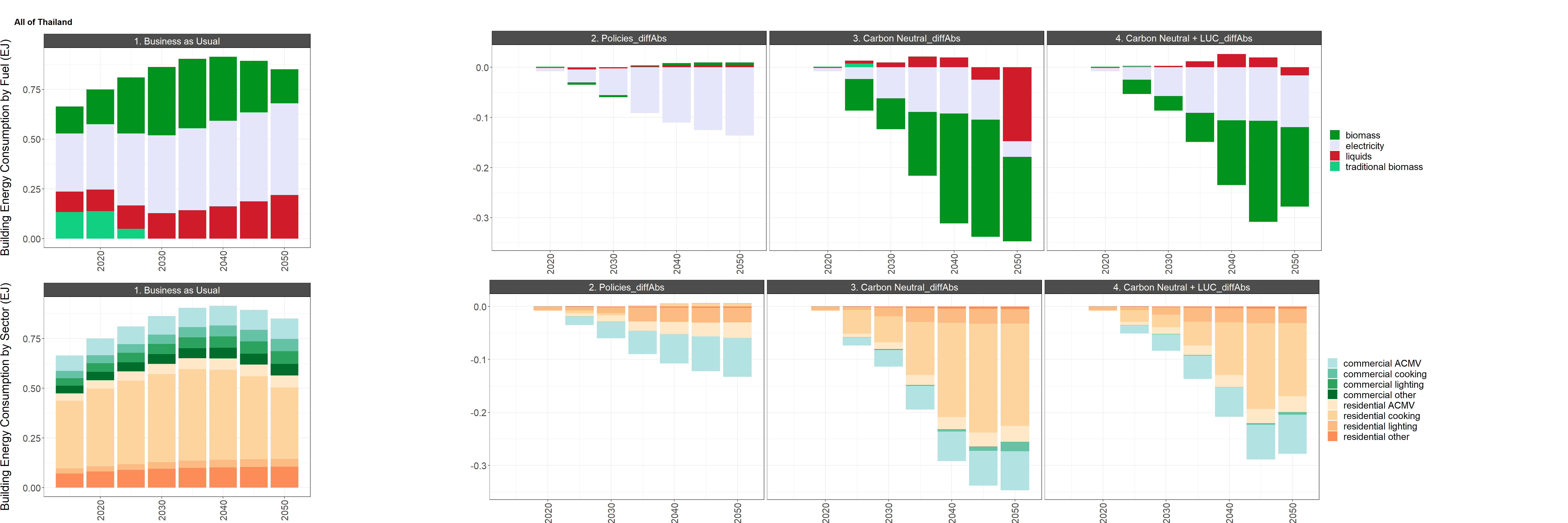

Difference in national buildings sector GHG emissions by service, final energy by fuel, and final energy by service between the reference scenario (left) and the low and high policy scenarios (right)

6.3.1.2.2 Transportation

transport_params <- c("transportFreightVMTByFuel", "transportPassengerVMTByFuel",
                      "transportPassengerVMTByTech", "transportFreightVMTByTech")

transport <- thailand %>% 
  filter(param %in% transport_params,
         region %in% c("All of Thailand", "MEA area"),
         !grepl("International", class)) %>%
  mutate(param = units) %>%
  rchart::chart(save = F, 
                show = F,
                size_text = 19,
                scenRef = scenRef_name,
                chart_type = c("class_absolute", "class_diff_absolute"),
                ncol = 4)

transport$`chart_class_All of Thailand`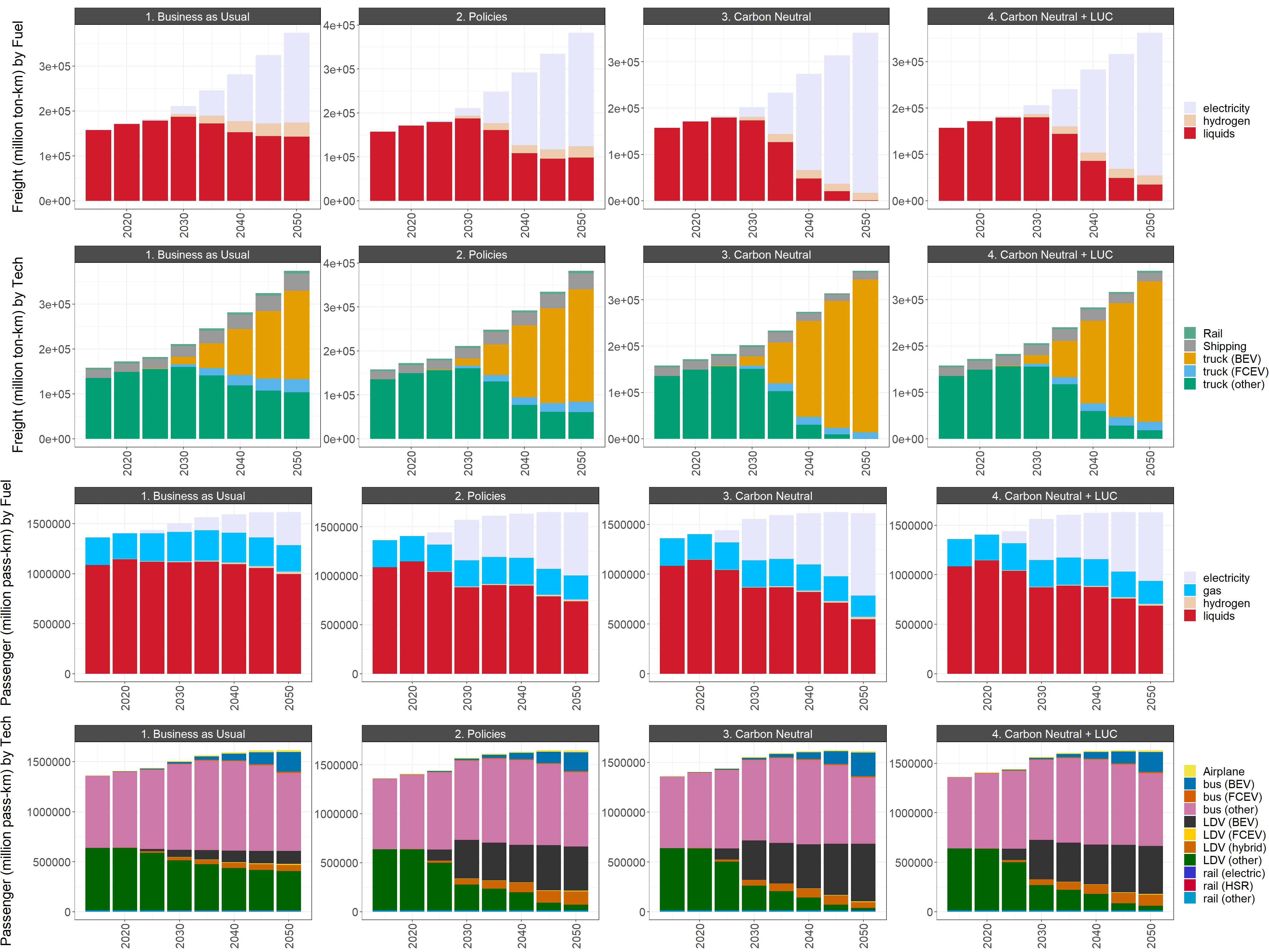

National transportation GHG emissions by mode and service output by mode and fuel in the reference scenario and the low and high policies scenarios

transport$`chart_class_diff_absolute_All of Thailand`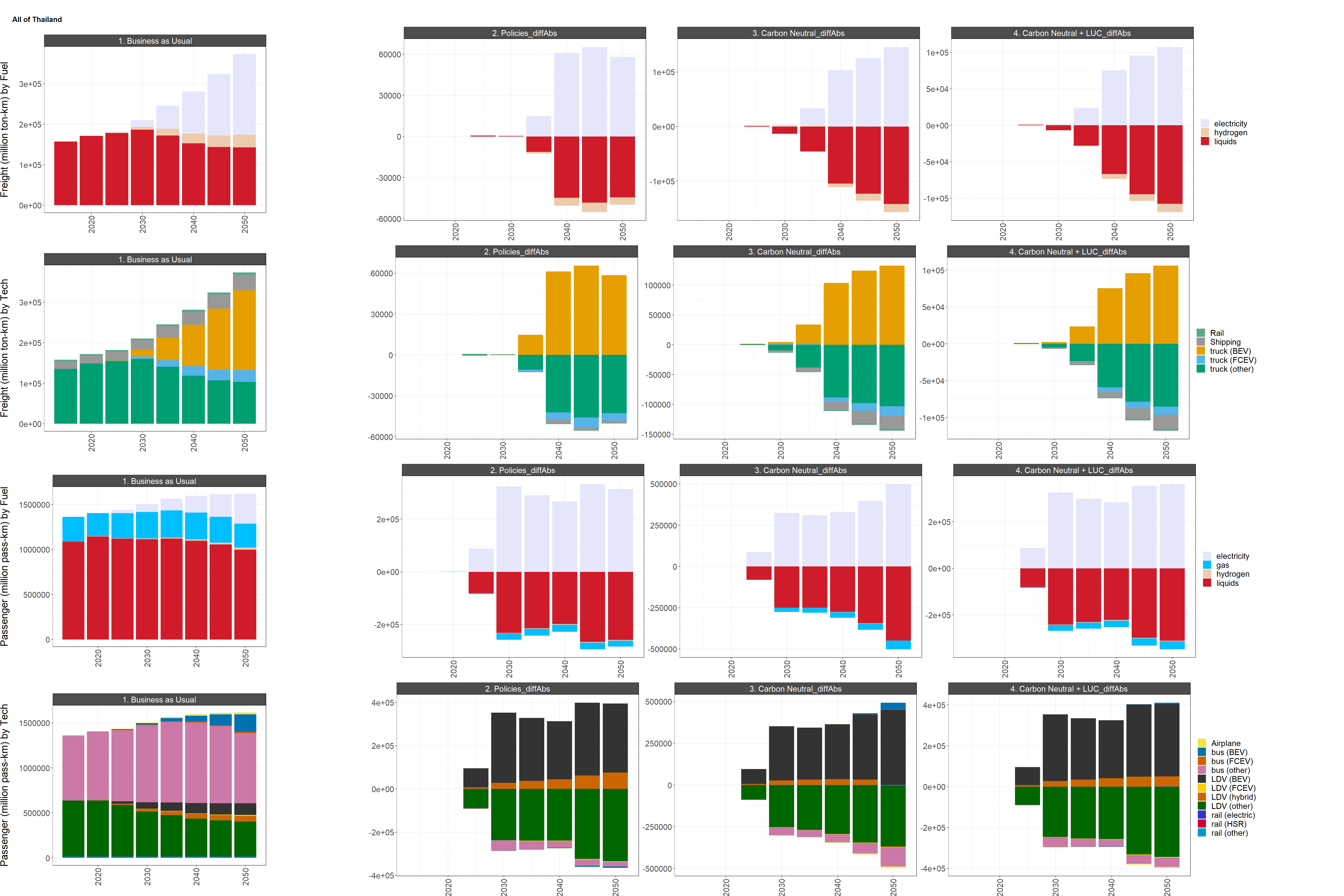

Difference in national transportation GHG emissions by mode and service output by mode and fuel between the reference scenario (left) and the low and high policy scenarios (right)

6.3.1.2.3 Industry

industry_params <- c("energyFinalSubsecByFuelIndusEJ")

industry <- thailand %>% 
  filter(param %in% industry_params,
         region %in% c("All of Thailand", "MEA area"),
         !class %in% c("biomass", "industrial feedstocks", "industrial processes")) %>%
  mutate(param = units) %>%
  rchart::chart(save = F, 
                show = F,
                size_text = 19,
                scenRef = scenRef_name,
                chart_type = c("class_absolute", "class_diff_absolute"),
                ncol = 4)

industry$`chart_class_All of Thailand`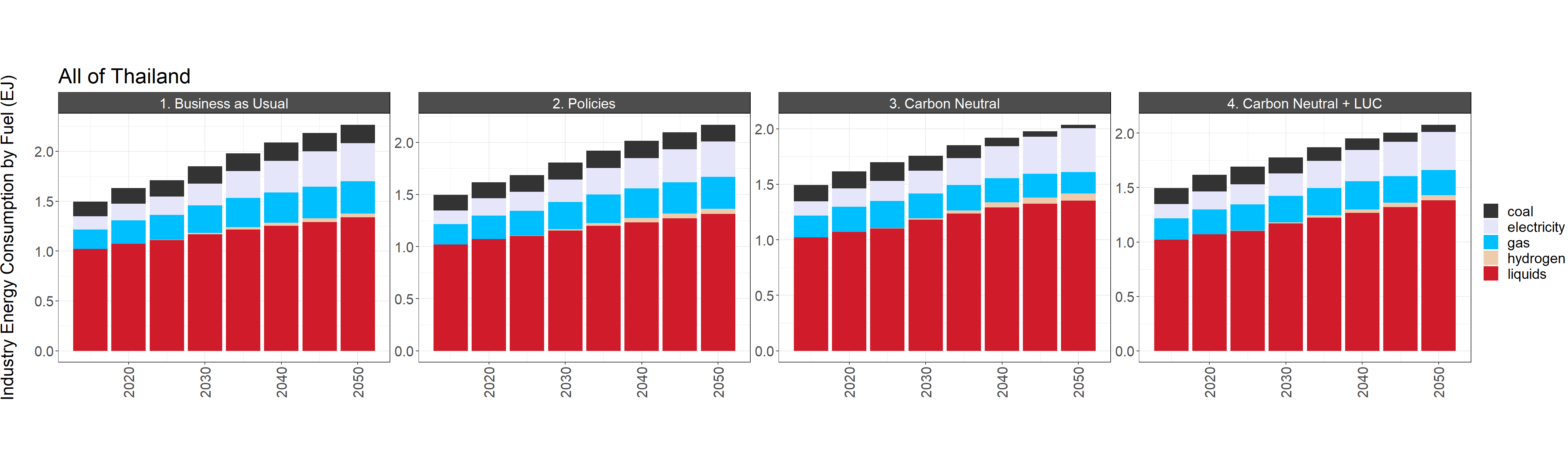

National industrial GHG emissions and final energy consumption by fuel in the reference scenario and the low and high policies scenarios

industry$`chart_class_diff_absolute_All of Thailand`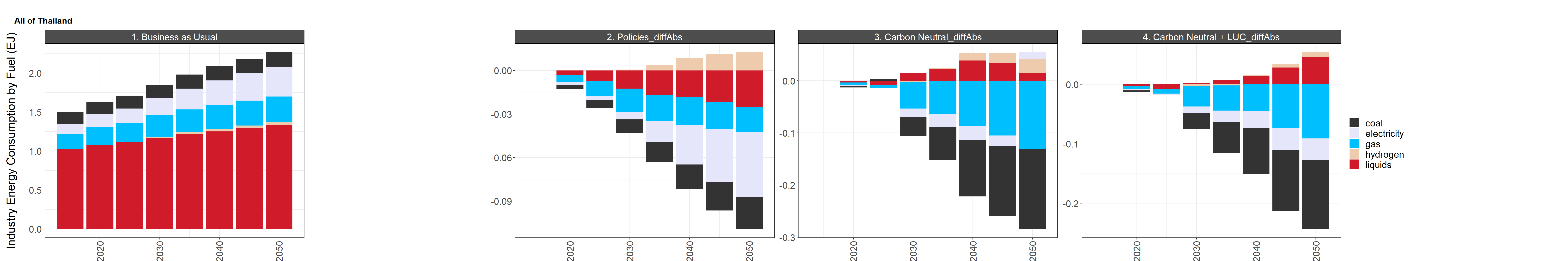

Difference in national industrial GHG emissions and final energy consumption by fuel between the reference scenario (left) and the low and high policy scenarios (right)

6.3.2 MEA Area

6.3.2.1 Summary figures

6.3.2.1.1 Socioeconomic summary

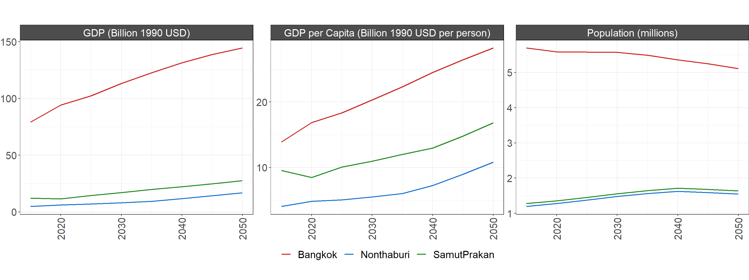
GDP, per capita GDP, and population in the MEA area from 2020 to 2065. Only the BAU scenario is shown since socioeconomic assumptions are consistent between scenarios.

6.3.2.1.2 Emissions by sector and gas

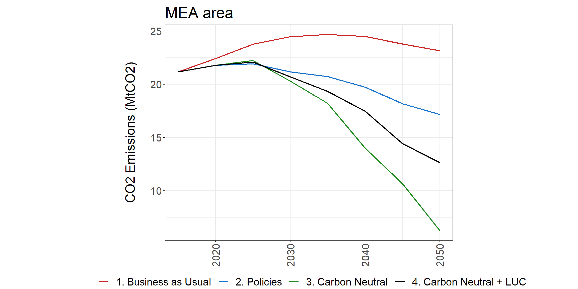
Total MEA area CO2 emissions (left) and GHG emissions (right) in the reference scenario and the low and high policies scenarios

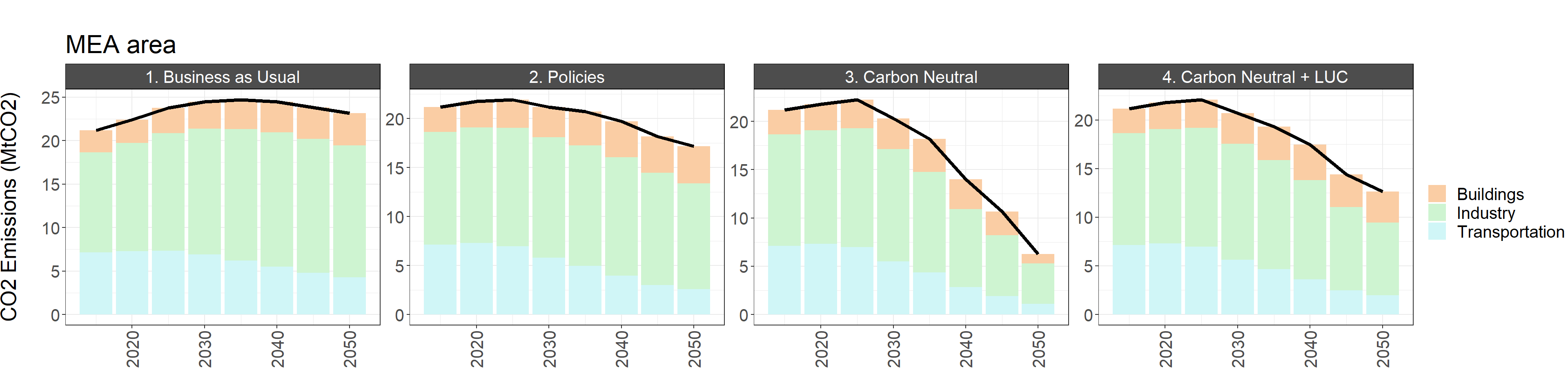
MEA area CO2 emissions by sector, GHG emissions by gas, and GHG emissions by sector in the reference scenario and the low and high policies scenarios

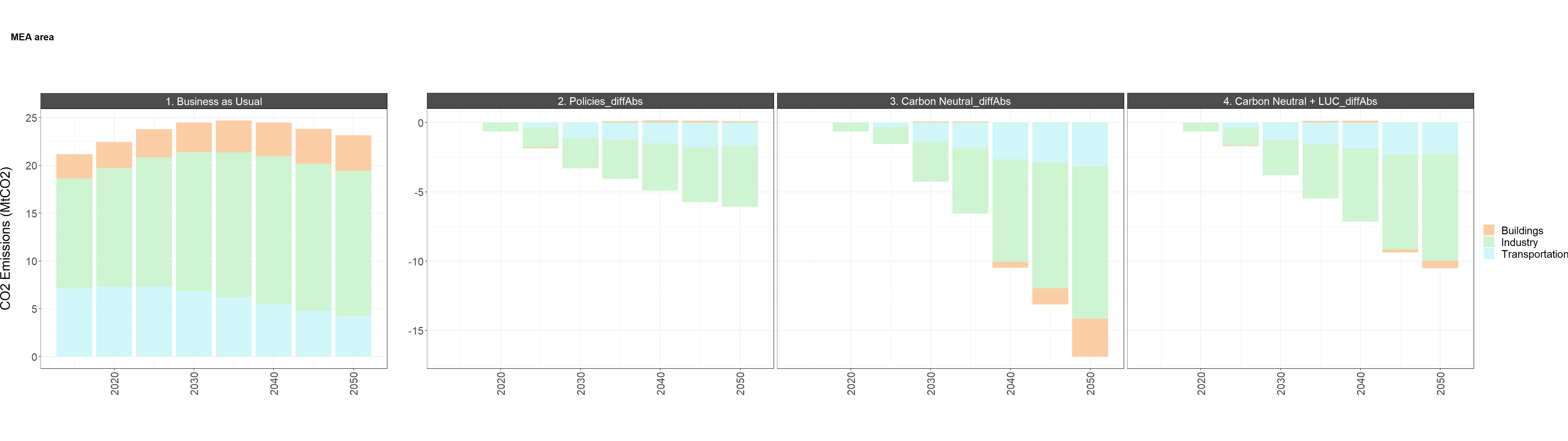
Difference in MEA area CO2 and GHG emissions by sector and gas between the reference scenario (left) and the low and high policy scenarios (right)

6.3.2.1.3 Final Energy by Fuel and Sector

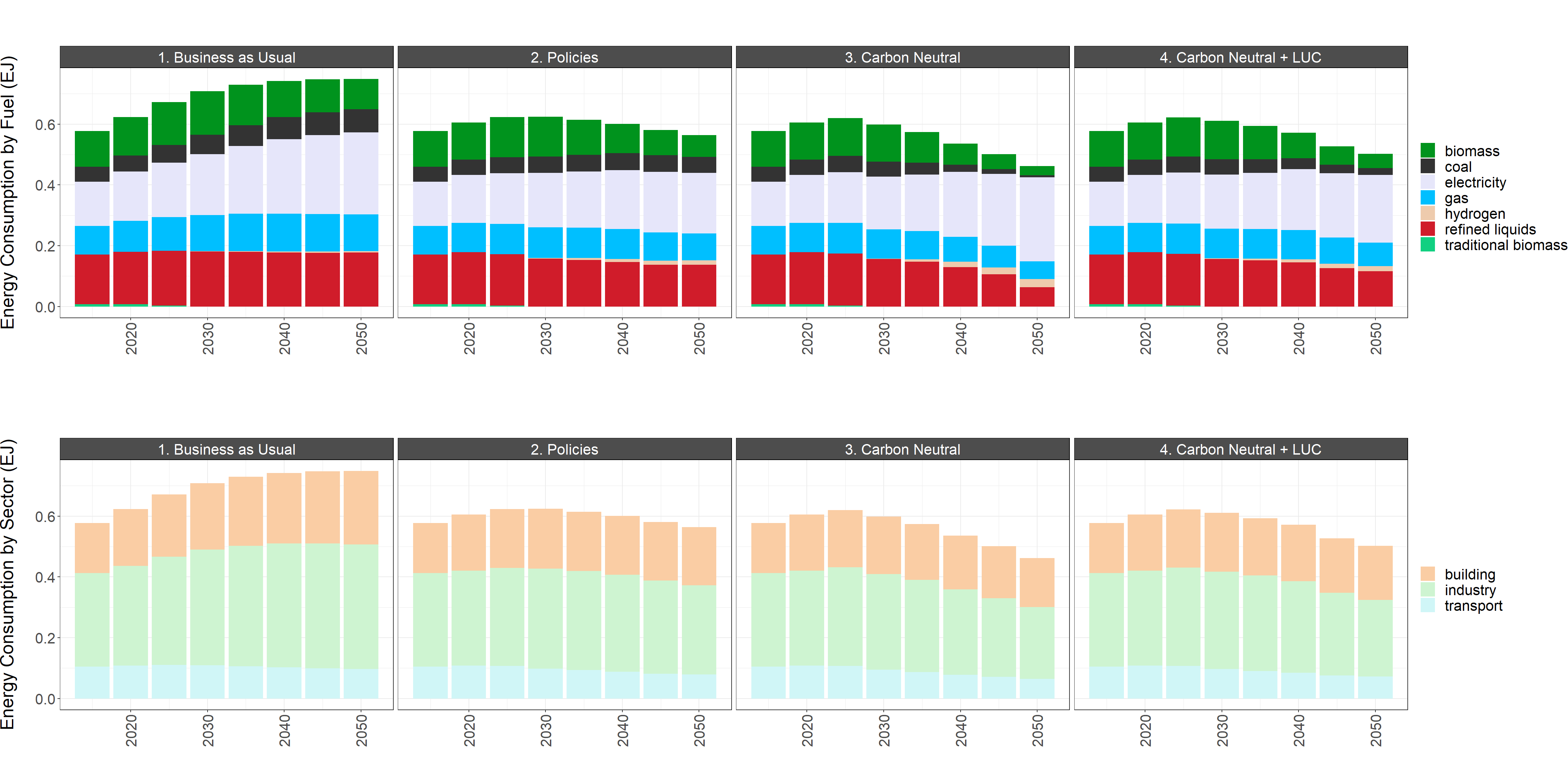
MEA area final energy consumption by fuel and sector in the reference scenario and the low and high policies scenarios

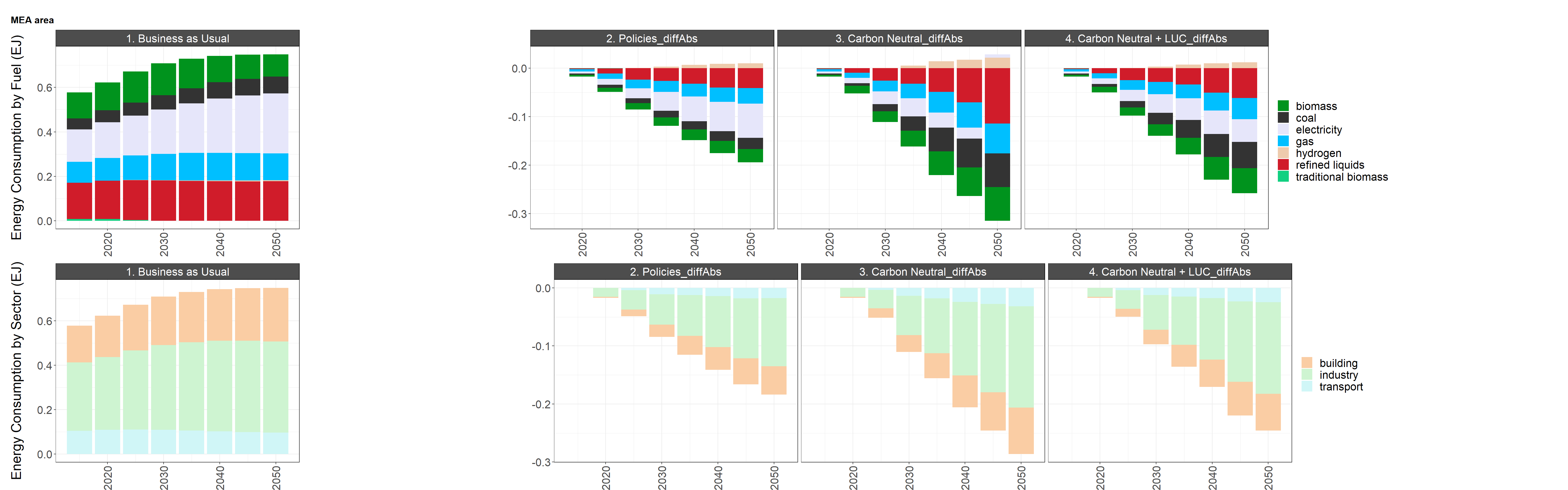
Difference in MEA area final energy consumption by fuel and sector between the reference scenario (left) and the low and high policy scenarios (right)

6.3.2.1.4 Electricity Consumption

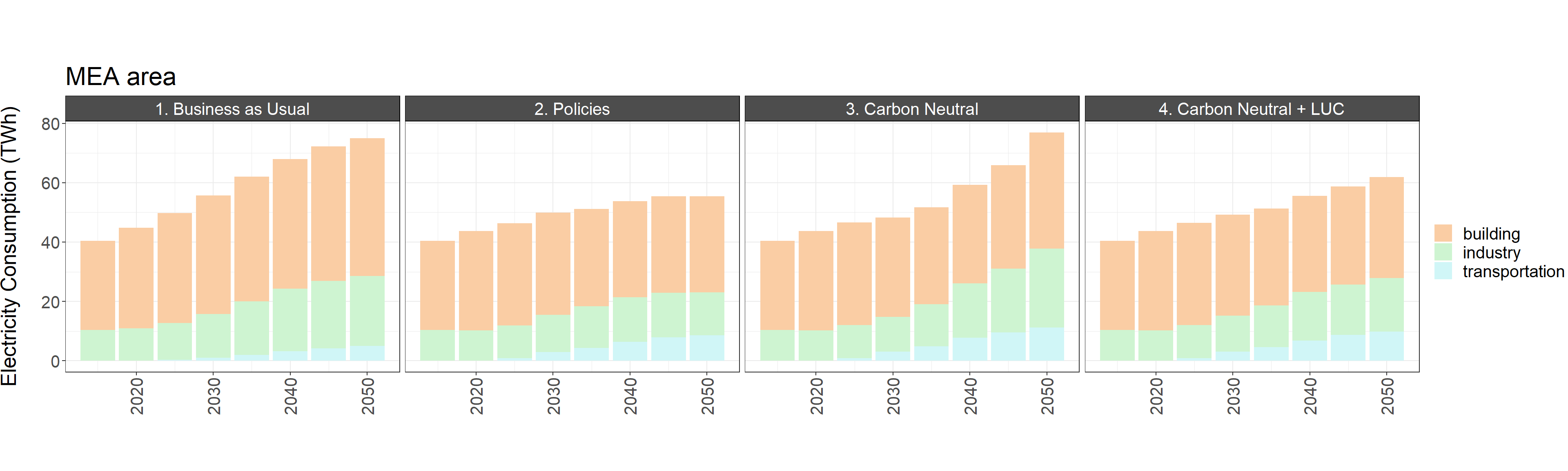
MEA area electricity generation by fuel, electricity consumption by sector, and power sector GHG emissions by gas and fuel in the reference scenario and the low and high policies scenarios

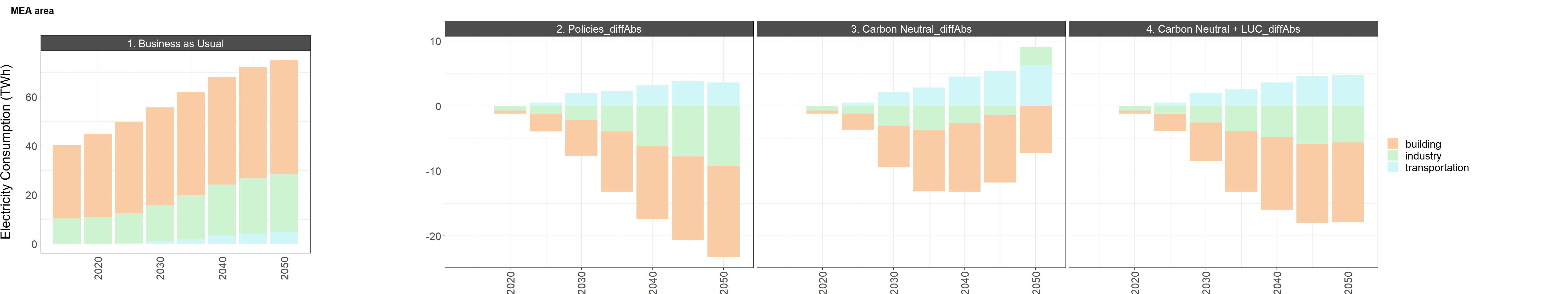
Difference in MEA area electricity generation by fuel, electricity consumption by sector, and power sector GHG emissions by gas and fuel between the reference scenario (left) and the low and high policy scenarios (right)

6.3.2.2 Sectoral details

6.3.2.2.1 Buildings

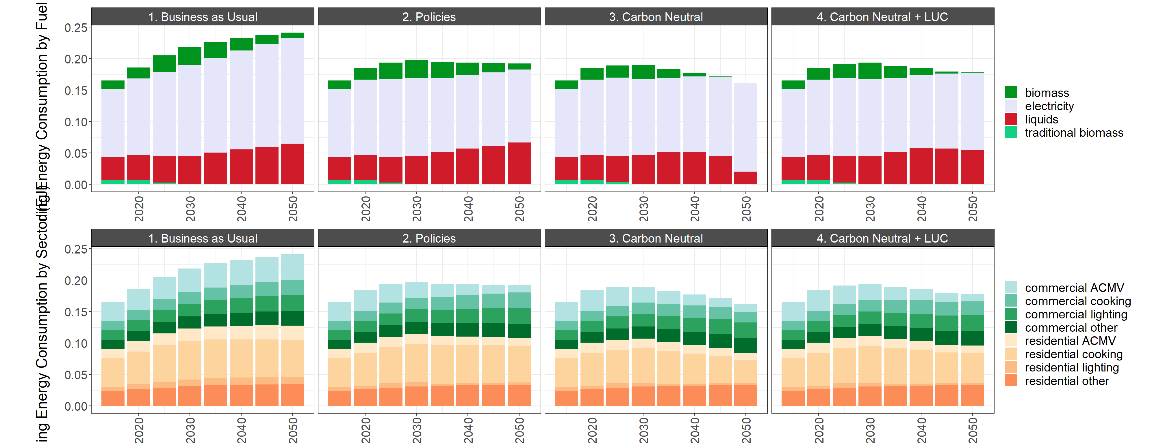
MEA area buildings sector GHG emissions by service, final energy by fuel, and final energy by service in the reference scenario and the low and high policies scenarios

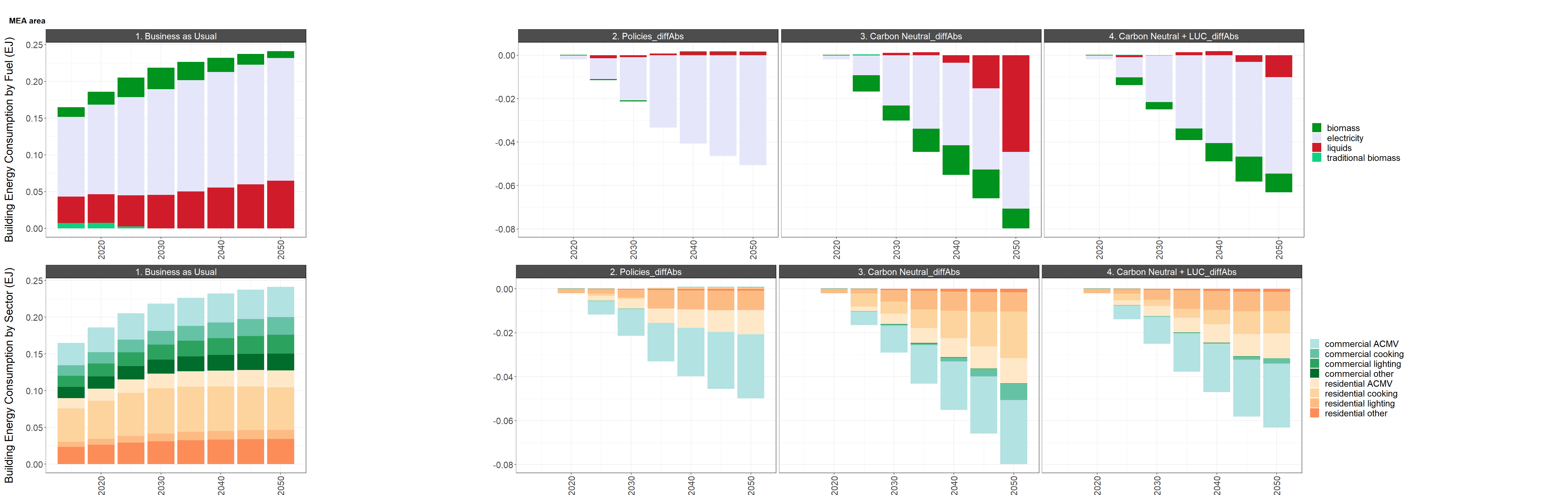
Difference in MEA area buildings sector GHG emissions by service, final energy by fuel, and final energy by service between the reference scenario (left) and the low and high policy scenarios (right)

6.3.2.2.2 Transportation

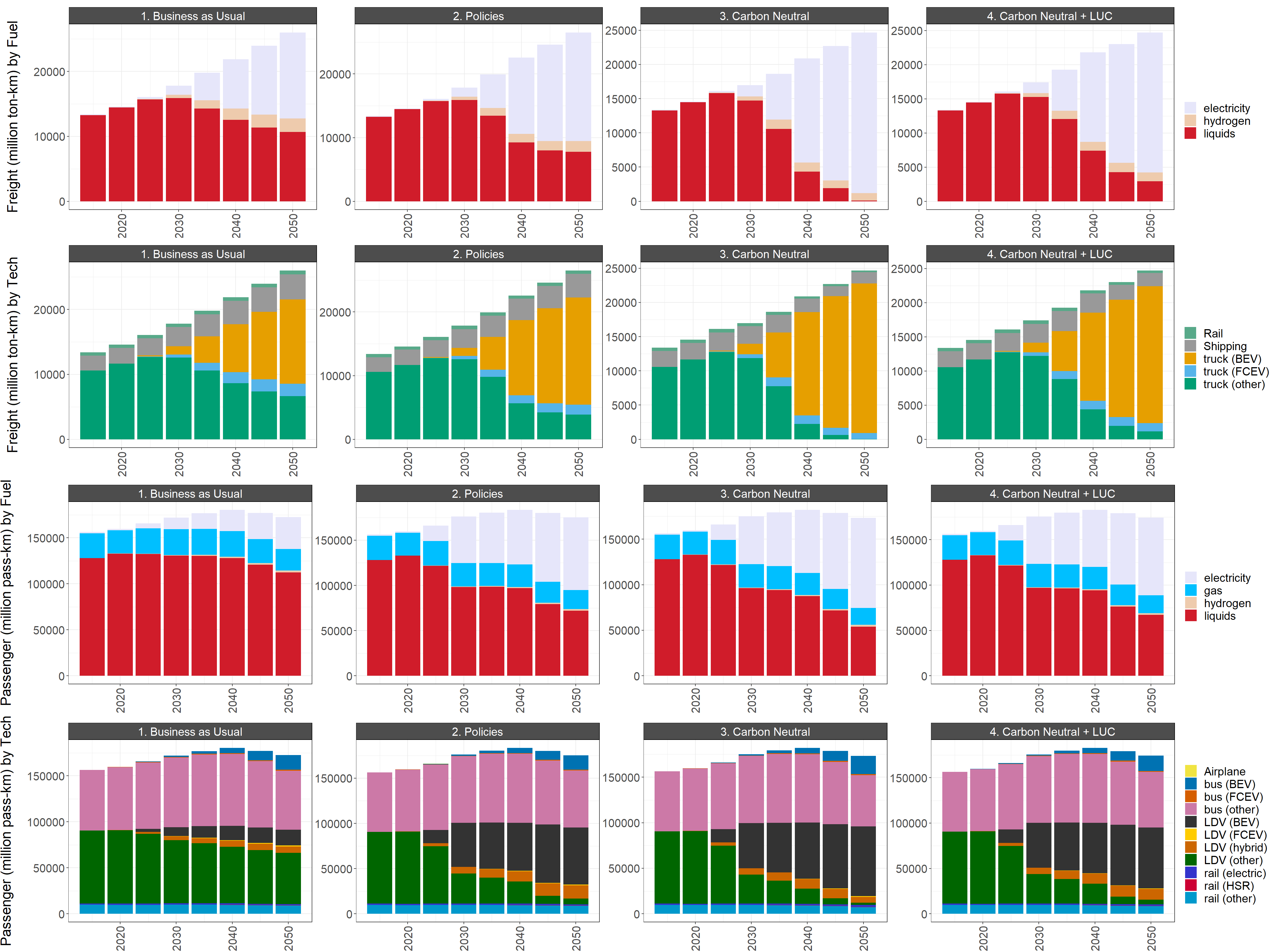
MEA area transportation GHG emissions by mode and service output by mode and fuel in the reference scenario and the low and high policies scenarios

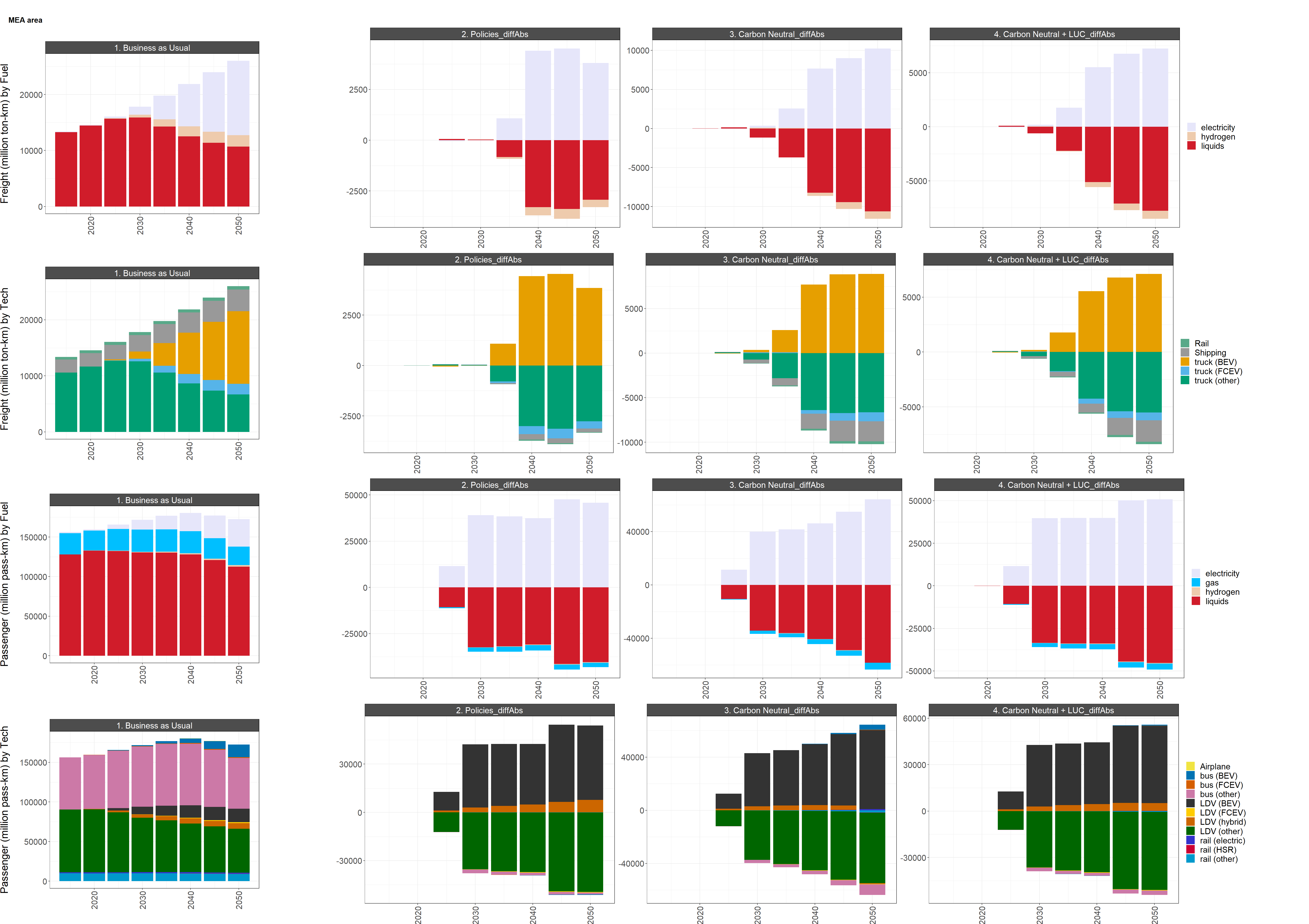
Difference in MEA area transportation GHG emissions by mode and service output by mode and fuel between the reference scenario (left) and the low and high policy scenarios (right)

6.3.2.2.3 Industry

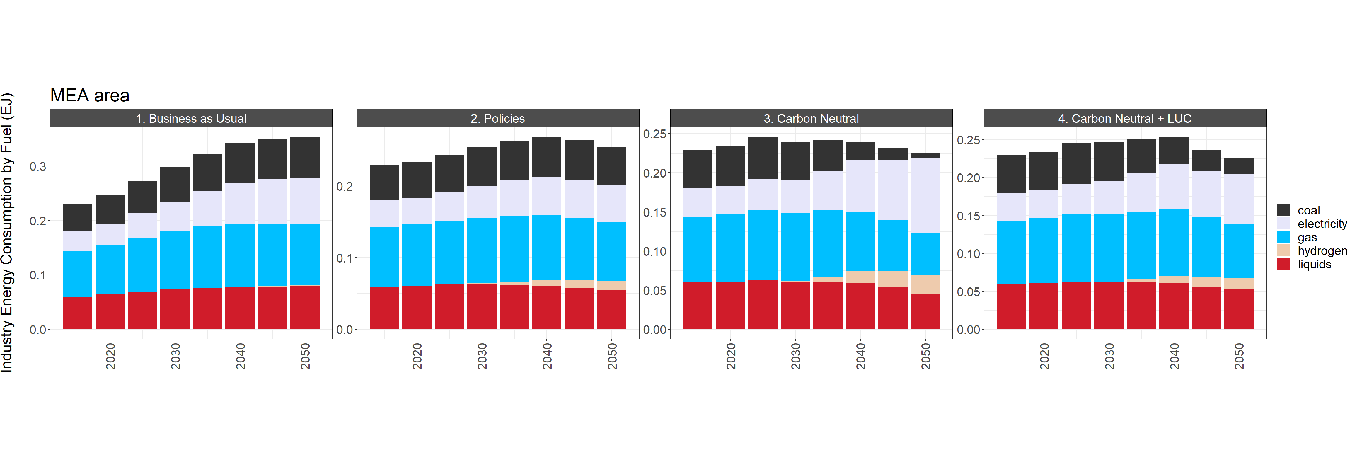
MEA area industrial GHG emissions and final energy consumption by fuel in the reference scenario and the low and high policies scenarios

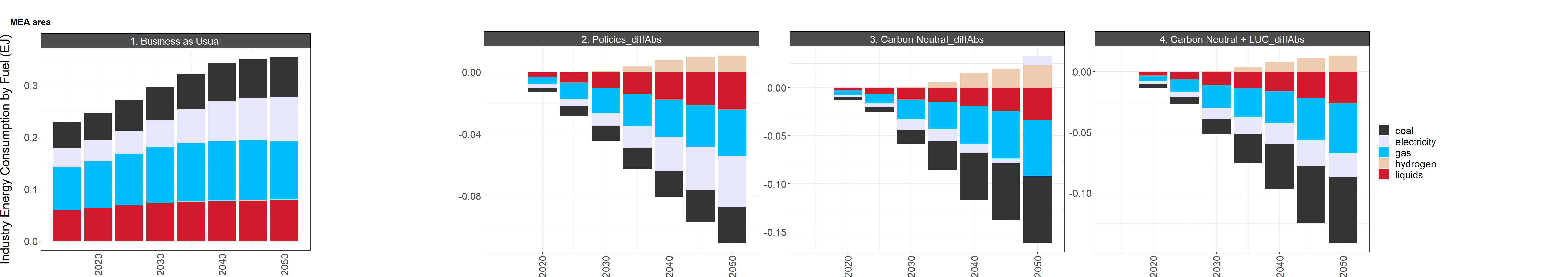
Difference in MEA area industrial GHG emissions and final energy consumption by fuel between the reference scenario (left) and the low and high policy scenarios (right)

7 Assumptions and Validation

7.1 Socioeconomic assumptions

This section describes the socioeconomic (population and GDP) inputs used to define Thailand’s subregions (Bangkok, Nonthaburi, Samut Prakan, and Rest of Thailand) in GCAM. Historical data were available from 1990 to 2020 for all regions, and projections published by local agencies were available for some future periods. The table below lists all data sources and assumptions.

Variable	Region	Data Sources	Assumptions
Population	National	- Historical (1993-2021): National Economic & Social Development Board (NESDB) - Projected (2022-2040): NESDB - Projected (2041-2100): United Nations (UN)	2041-2100 projection is from UN’s medium growth scenario.
Population	Provincial	- Historical (1993-2021): Department of Provincial Administration - Projected (2022-2040): NESDB	Post-2040 projections are based on shares of national population in 2040 (Bangkok: 8.1%; Nonthaburi: 2.5%; Samut Prakan: 2.6%).
GDP/GPP	National	- Historical (1990-2020): NESDB - Historical (2020-2021):Nikkei Asia article - Projected (2021-2050): missing link (NESDB)	Post-2050 national GDP projections follow assumption that GDP will be around 52,000 USD (2005) based on historical GDP per capita trends of developed nations.
GDP/GPP	Provincial	Historical (1995-2020): NESDB	GPP assumptions for 2021-2100 vary between provinces, with Bangkok’s per capita GDP reaching around 70,000 USD (2005) by 2100, consistent with income ranges of some high income cities at present.

The figures below show the time series produced for each region’s population, GDP, and per capita GDP based on the data sources and assumptions in the table:

7.1.1 Population

**Historical and projected future population in Thailand and MEA area. Sources: [NESDB](https://view.officeapps.live.com/op/view.aspx?src=https%3A%2F%2Fwww.nesdc.go.th%2Fewt_dl_link.php%3Fnid%3D3507%26filename%3Dsocial&wdOrigin=BROWSELINK) and [DOPA](https://stat.bora.dopa.go.th/new_stat/webPage/statByYear.php) (1990-2020), [NESDB](https://view.officeapps.live.com/op/view.aspx?src=https%3A%2F%2Fwww.nesdc.go.th%2Fewt_dl_link.php%3Fnid%3D3507%26filename%3Dsocial&wdOrigin=BROWSELINK) (2021-2040) and [United Nations](https://population.un.org/wpp/Download/Standard/Population/) (Post-2040)**

Historical and projected future population in Thailand and MEA area. Sources: NESDB and DOPA (1990-2020), NESDB (2021-2040) and United Nations (Post-2040)

7.1.2 GDP

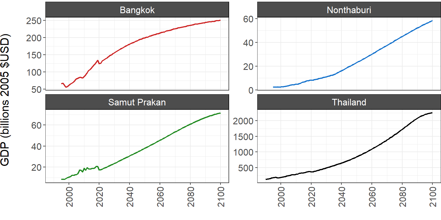
Historical and projected future GDP in Thailand and GPP in the MEA provinces.

7.1.3 Per Capita GDP

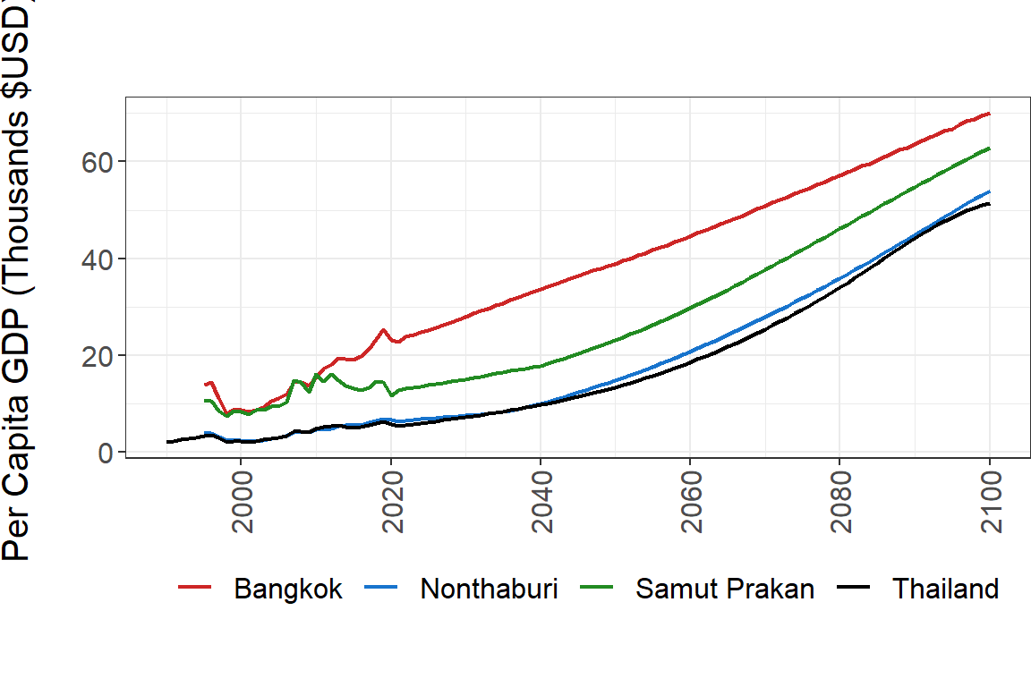
Thailand per capita GDP from 1990 to 2100 in constant 2005 $USD

7.2 Validation of GCAM outputs in historical periods

7.2.1 Thailand

7.2.1.1 Emissions

The following figures compare the GCAM output for Thailand’s CO2 emissions (total and by sector) to data from EPPO in historical years. The “Ref” GCAM scenario includes emissions from international shipping and aviation, while the “Ref-domestic” scenario does not.

National total CO2 emissions from 1986 to 2100 (left) and 1986 to 2015 (right) from GCAM output (blue) and local data (red). Local data source: Energy Policy and Planning Office

National total CO2 emissions by sector from local data (left) and GCAM output (right) from 2005 to 2015. Local data source: Energy Policy and Planning Office

7.2.1.2 Electricity

National electricity consumption from 2005 to 2100 (left) and 2011 to 2020 (right) from GCAM output (blue) and local utilities data (red). Local data source: Energy Policy and Planning office

Figure National electricity consumption by sector in 2015 and 2020 from local utilities data (left) and GCAM output (right). Local data source: Energy Policy and Planning office

7.2.1.3 Energy

There is a large discrepancy in the industrial energy consumption reported by EEP2018 versus GCAM in historical years. One explanation could be that the EEP2018 does not account for energy from industrial feedstocks while GCAM does. Each figure below includes the default GCAM output (“Ref”) as well as a version of the GCAM output that does not include industrial feedstocks (“Ref- No Feedstocks”).

National total final energy from 1986 to 2100 (left) and 1986 to 2020 (right) from GCAM output (blue) and local data (red). Local data source: Energy Policy and Planning Office

National total final energy by sector from local data (left), GCAM output (middle), and GCAM output without industrial feedstocks (right) in 2015. Local data source: Energy Efficiency Plan 2018

There is a similar discrepancy between GCAM historical data and EPPO’s energy consumption by fuel data. One cause of this discrepancy could be that EPPO does not include biomass energy.

National total final energy by fuel from local data (left), GCAM output (middle), and GCAM output without industrial feedstocks (right) from 2005 to 2020. Local data source: Energy Policy and Planning Office

7.2.1.4 Transportation

7.2.2 MEA area

7.2.2.1 Electricity

We have only found local data in the MEA area for electricity consumption. The following plots compare this local data to the GCAM reference scenario for total electricity consumption and electricity consumption by sector. Note that industrial energy consumption is much higher in the GCAM output than the local data in both 2015 and 2020. We are currently allocating industrial shares to subregions based on GDP, but we plan to adjust this methodology to reflect the fact that the Bangkok metropolitan area has less industrial activities than non-metropolitan areas despite having a higher per capita GDP.

Electricity consumption in the MEA service area from 2005 to 2100 (left) and 2011 to 2020 (right) from GCAM output (blue) and MEA data (red). Local data source: Energy Policy and Planning office

Electricity consumption by sector in the MEA service area from MEA data (left) and GCAM output (right) in 2015 and 2020. Local data source: Energy Policy and Planning office

WORK IN PROGRESS - DO NOT CITE