1 Introduction

This page explores the modeling process in depth. First, we walk through how to install GCAM for Southeast Asia, and how to set up our scenarios. Then, we describe the policies modeled and their technical implementation in the model. Finally, we include several sets of figures and the code to replicate them.

2 Download GCAM SE Asia

Please use the link below to download GCAM.

File	Location
gcamv5p3_seasia	Link

You will need the following prerequisites in order to run GCAM. You will also need at least 8 GB of RAM on your computer.

Prerequisite	Link
Java 64	Install Java 64
R	Install R
RStudio	Install RStudio
Windows XML Maker	Install Windows XML Maker

3 Guides

Below are links to an overview and walk-through of GCAM.

Description	File
GCAM overview presentation	gcam_overview.pdf
GCAM walkthrough presentation	gcam_walkthrough.pdf

4 Scenarios

Below are links to configuration files for the three scenarios that we will be using. The Business as Usual scenario models a reference case with no policies imposed, or the result of no additional action now. The Policies scenario includes targets for power generation, buildings, industry, and transportation sourced from Malaysia and Kuala Lumpur policies and plans. The Carbon Neutral scenario uses the same policies, but with an additional emissions constraint specifying that Malaysia must reach carbon neutrality by 2050.

Description	File
Business as Usual Scenario	configuration_malaysia_bau.xml
Policies Scenario	configuration_malaysia_policies.xml
Carbon Neutral Scenario	configuration_malaysia_carbon_neutral.xml

5 Policies

The policies modeled in the Policies and Carbon Neutral scenarios were sourced from Malaysia and Kuala Lumpur policies and plans. The table below details policies by sector with key values and targets as well as the source document/s (click to enlarge, click again to return to the main page).

Sets of policies modeled

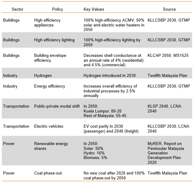
The following subsections give additional technical details and explanations for the policies listed above.

5.1 High Efficiency Appliances

Scenario	Files Used	Description
Policies, Carbon Neutral	buildings_efficient_appliances.xml	Increase prevelance of high-efficiency technologies through 2050

Goal

The goal of this policy is to represent an increase in energy efficient technologies in the building sector.

Approach

We can adjust the shareweights for technologies like air conditioners, water heaters, and other appliances to encourage the use of high efficiency technologies and discourage the use of low efficiency appliances.

Background - Share weights

Share weights are assigned to different subsectors and technology choices in GCAM to represent non-cost factors of consumer choice. They are used primarily to calibrate market shares to historical data but can also be modified to reflect factors such as infrastructure development or shifting societal preferences. For more information on share weights and how they are used in GCAM’s economic choice functions, see the GCAM economic choice documentation. Share weights should not be used to represent cost-related policies. Additionally, shareweight interpolation rules (fixed, linear, or s-curve) can be used to automatically interpolate shareweights between given years.

GCAM Implementation

Create a folder in the input directory: ./gcam-core/input/addons.
Download the “buildings_efficient_appliances.xml” file to the folder.
To adjust the year in which the target mix of technologies is achieved: within each stub-technology tag in the XML, change the to-year in the first interpolation-rule and the from-year in the second. Also change the year of the period tag in which the share-weight is 0.
Save the xml and then point to it in your configuration file by adding the line: <Value name = "scen">../input/addons/malaysia/buildings_efficient_appliances.xml</Value>

5.2 Lighting Efficiency

Scenario	Files Used	Description
Policies, Carbon Neutral	buildings_led.xml	Gradually phases non-LED residential lighting technology out of the market by 2050

Goal

The goal of this policy is to represent increasing use of LED lighting in residential buildings and the decreasing use of other less energy efficient lighting technologies.

Approach

We can gradually decrease the shareweights of all non-LED residential lighting technologies in order to phase them out of the market. The year in which the non-LED shareweights reach 0 corresponds with the year in which 100% LED residential lighting is achieved.

Background - Share weights

GCAM Implementation

Create a folder in the input directory: ./gcam-core/input/addons.
Download the “buildings_led.xml” file to the folder.
To adjust the year in which 100% LED lighting is achieved: within each non-LED stub-technology tag in the XML, change the to-year in the first interpolation-rule and the from-year in the second. Also change the year of the period tag in which the share-weight is 0.
Save the xml and then point to it in your configuration file by adding the line: <Value name = "scen">../input/addons/malaysia/buildings_led.xml</Value>

5.3 Building Envelope Efficiency

Scenario	Files Used	Description
Policies, Carbon Neutral	buildings_shell_eff.xml	Decreases shell conductance from 3.75 in 2020 to 0.487 (residential) / 0.375 (commercial) in 2070 at an annual rate of 4% (residential) / 4.5% (commercial)

Goal

The goal of this example is to represent increasing compliance with the envelope efficiency component of building energy codes.

Approach

We can use GCAM’s shell-conductance parameter to represent an increase in the average building envelope efficiency according to building energy codes.

Background - Cooling Demand

Cooling demand in GCAM depends on the indoor-outdoor temperature difference (measured using cooling degree days or CDD), the building’s shell conductance, and the building’s external heat gains along with GDP and price factors. For more details and to view the equation used to calculate cooling demand, see the Building service demand section of the GCAM energy demand documentation. GCAM’s shell-conductance parameter is the inverse of building envelope efficiency. Its units are watts per square meter per degree Kelvin and it represents the amount of heat transferred through the building’s exterior when there is a difference between the indoor and outdoor temperature.

GCAM Implementation

Create a folder in the input directory: ./gcam-core/input/addons.
Download the “buildings_shell_eff.xml” file to the folder.
To make custom adjustments: within each gcam-consumer tag in the XML, specify the desired shell-conductance values for each year.
Save the xml and then point to it in your configuration file by adding the line: <Value name = "scen">../input/addons/malaysia/buildings_shell_eff.xml</Value>

5.4 Hydrogen in Industry

Scenario	Files Used	Description
Policies, Carbon Neutral	industry_h2.xml	Phases hydrogen industrial technologies into the market in 2030

Goal

The goal of this policy is to represent a phase-in of industrial technologies that use hydrogen as a fuel source.

Approach

To represent a phase-in of hydrogen technologies, we can gradually increase their shareweights.

Background - Share weights

GCAM Implementation

Create a folder in the input directory: ./gcam-core/input/addons.
Download the “industry_h2.xml” file to the folder.
To adjust how quickly hydrogen technologies are phased into the market: within each subsector tag in the XML, change the to-year in the interpolation-rule. Also change the year of the period tag in which the share-weight is 1. Be sure that these years match. An earlier year corresponds to a faster phase-in.
Save the xml and then point to it in your configuration file by adding the line: <Value name = "scen">../input/addons/malaysia/industry_h2.xml</Value>

5.5 Industry Energy Efficiency

Scenario	Files Used	Description
Policies, Carbon Neutral	industry_aeei.xml	Increases overall efficiency of industrial processes by 2.5% annually through 2070

Goal

The goal of this policy is to represent measures to increase average efficiency of industrial processes.

Approach

To represent a gradual increase in industrial efficiency, we can use GCAM’s aeei parameter, which controls the autonomous energy efficiency improvement (AEEI) of industrial processes.

GCAM Implementation

Create a folder in the input directory: ./gcam-core/input/addons.
Download the “industry_aeei.xml” file to the folder.
To adjust the rate of industrial energy efficiency increase, change the value of the aeei tag for each desired year.
Save the xml and then point to it in your configuration file by adding the line: <Value name = "scen">../input/addons/malaysia/industry_aeei.xml</Value>

5.6 Public/Private Vehicle Modal Shift

Scenario	Files Used	Description
Policies, Carbon Neutral	trn_modal_shift.xml	Increases ratio of public to private transportation to 80-20 in Kuala Lumpur and 55-45 in the rest of the country in 2050

Goal

The goal of this policy is to increase the shares of public transportation methods relative to private transportation.

Approach

To represent a transition to public transportation, we adjust the shareweights of public transportation modes (Bus, Rail, Walk, and Cycle) in Kuala Lumpur and the Rest of Malaysia in order to increase their share in the market.

GCAM Implementation

Create a folder in the input directory: ./gcam-core/input/addons.
Download the “trn_modal_shift.xml” file to the folder.
To make custom adjustments, change the share-weight for year="2100" in a given tranSubsector. Increasing the share-weight will result in a greater share of the mode that was adjusted, while decreasing it will result in less.
Save the xml and then point to it in your configuration file by adding the line: <Value name = "scen">../input/addons/malaysia/trn_modal_shift.xml</Value>

5.7 EV Cost Parity

Scenario	Files Used	Description
Policies, Carbon Neutral	trn_ev_cost_parity.xml	Reduces EV costs to reach cost parity with liquids vehicles by 2030 (passenger) and 2040 (freight)

Goal

The goal of this policy is represent measures to make EVs more competitive with combustion engine vehicles (CEV).

Approach

To represent EV promotion, we use an approach that decreases the cost of EVs relative to CEVs, until the two technologies reach cost parity in some future year. We can do this using GCAM’s input-cost parameter, which represents the non-energy costs of a given technology.

Background - Transportation Cost

In GCAM, the costs of different transportation technologies are comprised of two components: fuel costs and non-fuel costs. A transportation technology’s fuel cost is determined by its vehicle fuel intensity as well as fuel price. The non-fuel costs encompass factors such as capital costs, operation and maintenance, and service costs. These non-fuel costs can be adjusted using the input-cost parameter. For more information on how transportation demand is modeled in GCAM, including cost calculations, see the transportation sections of the GCAM Demand for Energy documentation.

GCAM Implementation

Create a folder in the input directory: ./gcam-core/input/addons.
Download the “trn_ev_cost_parity.xml” file to the folder.
To make custom adjustments to the EV cost trajectory, set the desired input-cost for each year within eachstub-technology tag in the cost parity xml file.
Save the xml and then point to it in your configuration file by adding the line: <Value name = "scen">../input/addons/malaysia/trn_ev_cost_parity.xml</Value>

5.8 Electricity Generation Mix

Scenario	Files Used	Description
Policies, Carbon Neutral	elec_gen_shares.xml	Sets shares for renewable electricity generation technologies
Policies, Carbon Neutral	elec_hydro.xml	Sets exogenous hydropower generation

Goal

The goal of this example is to set a share for the amount of electricity generation from two renewable energy technologies (solar and biomass) corresponding with the planned percentages in the KLLCSBP2030 (below). Because hydropower is exogenous in GCAM, we set a generation value (in EJ) rather than a share.

Approach

One way to set a generation floor for each fuel type in GCAM is to use a subsidy policy. This will lower the cost of the electricity generation technology until the floor is reached. If there is more demand for electricity than is supplied by the sum of the generation floors, then the remaining demand will be met by a mix of fuels determined by the market.

Hydropower is exogenous in GCAM and has a fixed pathway. The power generation values for this technology are set explicitly using a fixed output add-on XML.

Background - Policy portfolio standards

A policy-portfolio-standard in GCAM is a policy that can be used to implement taxes, subsidies, floors, ceilings, and constraints. Taxes and subsidies can be specified when the exact amount to be added or subtracted to the price is known. However, a policy-portfolio-standard can also contain a constraint, which acts as either a floor or ceiling for the technology or technologies included. Exact constraints can also be implemented. See the GCAM Policy Examples documentation for more information on how to implement these options.

GCAM Implementation

Create a folder in the input directory e.g.. ./gcam-core/input/addons/malaysia.
Download the “elec_gen_shares.xml” file to the folder.
To make adjustments for generation sources currently included (solar, biomass): within each minicam-energy-input tag in the XML, adjust the current-coef for each year in which a floor is desired. The find + replace function is useful here due to the size of the XML.
To add a new generation source to set a share for

Create a policy-portfolio-standard for the technology (use current XML as an example).
Add this technology as a minicam-energy-input within each supplysector or pass-through-sector/subsector/stub-technology for every period, and adjust the current-coef.
Create a res-secondary-output for this technology, where applicable. For example, a res-secondary-output is created for solar in supplysector:electricity/subsector:solar/stub-technology:PV, supplysector:electricity/subsector:solar/stub-technology:PV_storage, supplysector:elect_td_bld/subsector:rooftop_pv/stub-technology:rooftop_pv, pass-through-sector:elec_CSP/subsector:CSP/stub-technology:CSP (recirculating), pass-through-sector:elec_CSP/subsector:CSP/stub-technology:CSP (dry_hybrid), pass-through-sector:elec_CSP_storage/subsector:CSP_storage/stub-technology:CSP_storage (recirculating), and pass-through-sector:elec_CSP_storage/subsector:CSP_storage/stub-technology:CSP_storage (dry_hybrid), because these are all solar-related technologies.

To adjust the hydropower pathway, download the “elec_hydro.xml” file to the folder.
Within each fixedOutput tag in the XML, adjust the value to reflect desired hydropower output in each period. The user can also add additional periods.
Save the XMLs and then point to them in your configuration file by adding the lines: <Value name = "scen">../input/addons/malaysia/elec_gen_shares.xml</Value> <Value name = "scen">../input/addons/malaysia/elec_hydro.xml</Value>

5.9 Coal Phase-Out

Scenario	Files Used	Description
Policies, Carbon Neutral	elec_no_new_coal.xml	Prevents additional coal capacity from being built starting in 2020
Policies, Carbon Neutral	elec_coal_shutdown.xml	Retires existing coal capacity; all coal is retired by 2050

Goal

The goal of this example is to phase out coal from Malaysia’s electricity generation capacity. Note that this policy only applies at the national level.

Approach

There are two steps to phase out coal generation. The first is to prevent any new coal capacity from being built; we do this by setting coal shareweights to 0 in all future years. The second step is to gradually retire all existing coal capacity; we do this by shortening coal technologies’ lifetimes and by assigning a shutdown curve to each technology.

Background - Share weights

Background - Energy Technology Retirement

For some energy technologies, such as coal, the “cohort” installed in each period is modeled as a separate technology. Therefore, even if no new capacity is installed in future years, output from the capacity installed in previous years will still be modeled. There are several GCAM parameters that determine the trajectory of output from previously installed technology cohorts. The lifetime is the maximum number of years for which the technology cohort can continue producing output; i.e., a technology cohort installed in year t will no longer produce any output in the year t + lifetime. The s-curve-shutdown-decider is a function that controls the speed at which the technology cohort retires, or reduces its output, within its lifetime. This function depends on a steepness parameter that determines the shape of the function as well as a half-life parameter that sets the number of years after which half of the technology cohort is retired. For more information on retirement parameters, see the GCAM Energy Technologies documentation.

GCAM Implementation

Create a folder in the input directory e.g.. ./gcam-core/input/addons.
Download the “elec_no_new_coal.xml” and “elec_coal_shutdown.xml” files to the folder.
To make custom adjustments to the coal retirement trajectory, optionally change the following within each stub-technology tag in the retirement XML:

Use lifetime to adjust the year in which the coal phase-out is complete; the phase-out will be complete x years after 2015, where x is the lifetime.
Use the steepness and half-life within the s-curve-shutdown-decider to adjust the phaseout trajectory; a smaller half-life and larger steepness will result in a faster phase-out.

Save the xmls and then point to them in your configuration file by adding the lines: <Value name = "scen">../input/addons/malaysia/elec_no_new_coal.xml</Value> <Value name = "scen">../input/addons/malaysia/elec_coal_shutdown.xml</Value>

6 Net-Zero & Carbon Netural

Scenario	Files Used	Description
Carbon Neutral	NetZeroC_Malaysia_2035_2050	CO2 emissions constraint for Malaysia (2035 - 2050)
Carbon Neutral	Malaysia_LUC	GHG link file for Malaysia for land use change emissions
Carbon Neutral	NetZeroC_global_noMalaysia_2050	CO2 emissions constraint for the rest of the World (2050)
Carbon Neutral	ROW_LUC_noMalaysia	GHG link file for land use change emissions for the rest of the world

Goal

The aim of this example is to demonstrate how to apply an economy-wide emissions constraint for Malaysia in accord with its national goals: net-zero CO₂ as early as 2050.

Approach

In GCAM, an emissions constraint can be accomplished by using a ghgpolicy, which is a special case of policy-portfolio-standard that applies to emissions.

Background

To implement a ghgpolicy in GCAM, users specify the total amount of emissions (CO₂ or GHG) in a time period. GCAM will then calculate the price on carbon needed to reach the constraint in each period. GCAM finds the least-cost pathway in terms of technology deployment to satisfy the emissions constraint. An economy-wide constraint can be used by itself, or in combination with additional sectoral policies described above.

There are some important considerations: (1) What GHGs are included in the constraint (e.g., only CO₂)?, (2) What is the time period for the constraint (e.g., 2050, 2065)?, (3) What are the emissions in each period?, (4) Will emissions decline linearly to zero or will another rate be specified?, (5) Will land use change emissions be included in the constraint?, and (6) What assumptions are made for emissions in the rest of the world? This latter point is important when considering “carbon leakage,” that is, how restrictions in emissions in one geography may lead to a shift in carbon-intensive activities to other locations. Below, we will describe how to implement a CO₂ emissions constraint. See the GCAM Policies documentation for more information.

GCAM Implementation

Create a folder in the input directory: ./gcam-core/input/addons.
Download the emissions constraint xml file(s) for Malaysia: “NetZeroC_Malaysia_2035_2050” and “Malaysia_LUC”, as well as those for the rest of the world (ROW), “NetZeroC_global_noMalaysia_2050” and “ROW_LUC_noMalaysia.”
The first file, NetZeroC_Malaysia_2035_2050, specifies emissions in units of tonnes of carbon (not CO₂) in each period. One way to determine the emissions constraint for each period is to examine the CO₂ emissions in the reference case (See ModelInterface: “CO₂ emissions by region”). Based on the reference emissions, one can create an emissions constraint accordingly, depending on the start date of the emissions constraint, end goal, and steepness of the decrease in emissions.
You will notice that the constraint starts in 2035. We want to first incorporate the pathway for Malaysia’s Nationally Determined Contribution (NDC) from 2020 to 2030. Malaysia’s NDC includes a target to reduce its greenhouse gas (GHG) emissions intensity of GDP by 45% by 2030 relative to the emissions intensity of GDP in 2005. When we examine GHG emissions (See ModelInterface: “nonCO₂ emissions by region”) and GDP (See ModelInterface: “GDP MER by region”), we see that this target is met without any additional policy in the reference scenario. Thus, we only need to start our constraint in 2035. We specify a linear decrease to 0 tonnes of C in 2050.
We adopt a similar approach for the ROW, using the total emissions (tC) in 2020 for all countries as a starting point. (We did not subtract out Malaysia’s emissions, as they are quite small globally). It is not absolutely necessary to adopt the very same emissions constraint for the ROW, but the constraint should be strong enough to avoid carbon leakage from Malaysia’ net-zero policy.
One needs to decide whether and how land use change emissions are incorporated into the constraint. GCAM accounts for fossil fuel and industry CO₂ emissions separately from land use change CO₂ emissions. The Malaysia_LUC.xml specifies how land use change CO₂ emissions (LUC-CO₂) in Malaysia are linked to the ghgpolicy (“CO₂”). There are two parameters: price-adjust and demand-adjust. Price-adjust is used to convert prices for different GHGs. A price-adjust of 1.0 for LUC-CO₂ means the market price on LUC-CO₂ emissions is the same as the price applied to fossil fuel and industry CO₂ emissions. A demand-adjust of 1 means that LUC-CO₂ emissions are counted in the emissions constraint. These two parameters can be adjusted. In the sample files we have a price-adjust of 0, and a demand-adjust of 1. This can be modified depending on the goal and importance of LUC emissions. Note that Malaysia is removed from the ROW_LUC_noMalaysia.xml.
Save the xml files and then point to them in your configuration file by adding the lines: <Value name = "scen">../input/addons/malaysia/NetZeroC_Malaysia_2035_2050.xml</Value> <Value name = "scen">../input/addons/malaysia/Malaysia_LUC.xml</Value> <Value name = "scen">../input/addons/malaysia/NetZeroC_global_noMalaysia_2050.xml</Value> <Value name = "scen">../input/addons/malaysia/ROW_LUC_noMalaysia.xml</Value>

7 Diagnostics

This section describes how to explore and compare the final output data using GCAM-specific post-processing tools.

7.1 Extract GCAM Data

gcamextractor is an R package used to extract and process GCAM data and manipulate into standardized tables. gcamextractor converts GCAM outputs into commonly used units and aggregates across different classes and sectors for easy use in plots, maps, and tables. For more information, please reference the documentation page found here.

The first step is to create a path to the GCAM database, found in the output folder of your GCAM folder, and a list of desired parameters. The readgcam() function also requires region names and a specific output folder. Note that due to size limitations on GitHub, the data used here has already been processed, but we include the steps to run it on your own in the following chunk if desired.

# Get desired database paths
bau_db <- "../data/malaysia/output/malaysia_bau"
policies_db <- "../data/malaysia/output/malaysia_policies"
carbon_neutral_db <- "../data/malaysia/output/malaysia_carbon_neutral"

paths <- c(bau_db, policies_db, carbon_neutral_db)

# Choose parameters of interest
params <- c("elecByTechTWh", 
            "emissCO2BySectorNoBio", 
            "energyFinalByFuelEJ", 
            "energyFinalConsumBySecEJ", 
            "energyFinalSubsecBySectorBuildEJ", 
            "energyFinalSubsecByFuelBuildEJ",
            "energyFinalSubsecByFuelIndusEJ",
            "energyFinalByFuelTransportPassEJ",
            "energyFinalByFuelTransportFreightEJ"
            "transportFreightVMTByMode", 
            "transportPassengerVMTByMode",
            "gdp", "gdpPerCapita", "pop")

# Identify regions
regions <- c("Malaysia", "KualaLumpur", "Rest of Malaysia")

# Loop through each database to get gcamextractor output
for(p in paths){
  gcamextractor::readgcam(gcamdatabase = p,
                          regionsSelect = regions,
                          regionsAggregate = list(regions),
                          regionsAggregateNames = "All of Malaysia",
                          paramsSelect = params,
                          folder = paste0("../data/malaysia/gcamextractor/", tail(strsplit(p, "/")[[1]],1)))
}

# Read in data
bau <- read.csv("../data/malaysia/gcamextractor/malaysia_bau/gcamDataTable_aggClass1.csv") 
policies <- read.csv("../data/malaysia/gcamextractor/malaysia_policies/gcamDataTable_aggClass1.csv")
carbon_neutral <- read.csv("../data/malaysia/gcamextractor/malaysia_carbon_neutral/gcamDataTable_aggClass1.csv")

# Combine data into one data frame
malaysia <- bind_rows(bau, policies, carbon_neutral) %>%
  filter(region != ("Rest of Malaysia"),
         x > 2000, x <= 2050)

# Reorder scenarios
malaysia$scenario <- factor(malaysia$scenario, 
                            levels = c("Ref", "High", "High_CarbonNeutral"),
                            labels = c("1. Business as Usual", "2. Policies", "3. Carbon Neutral"))

# Define reference scenario
REF_SCENARIO <- "1. Business as Usual"

# Use this to access reference scenario plot
c <- paste0("chart_class_", REF_SCENARIO)

7.2 Plot Figures

rchart is a comprehensive charting package to plot and compare data across scenarios, regions, sectors and time periods in GCAM. The diagnostic figures below were created using gcamextractor and rchart and include the following parameters:

Socioeconomics: population, GDP, GDP per capita
CO₂ emissions by sector
Final energy by fuel
Final energy by sector
Electricity generation by fuel
Building energy by subsector
Transportation by mode
Transportation by fuel
Industry energy by fuel

To enlarge a figure, please click directly on the image. Click on the image again to close out.

7.2.1 Summary Figures

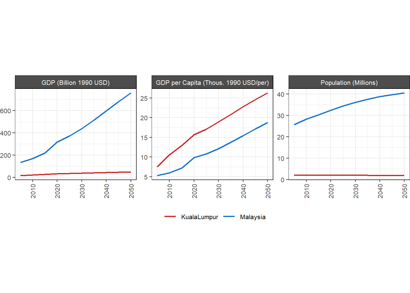
7.2.1.1 Socioeconomic Summary

figure_path <- "./markdown_figs"

socioeconomic_parameters <- c("pop", "gdp", "gdpPerCapita")

socioeconomic <- malaysia %>%
  filter(param %in% socioeconomic_parameters,
         region != "All of Malaysia",
         scenario == REF_SCENARIO) %>%
  mutate(param = units,
         param = case_when(classLabel == "GDP Per Capita" ~ "GDP per Capita (Thous. 1990 USD/per)", T~param)) %>% 
  rchart::chart(save = F, 
                show = F,
                chart_type = "region_absolute",
                folder = figure_path,
                append = "_socioeconomics",
                size_text = 10)

socioeconomic$chart_region_absolute

BAU GDP, GDP per capita, and population in Malaysia and Kuala Lumpur

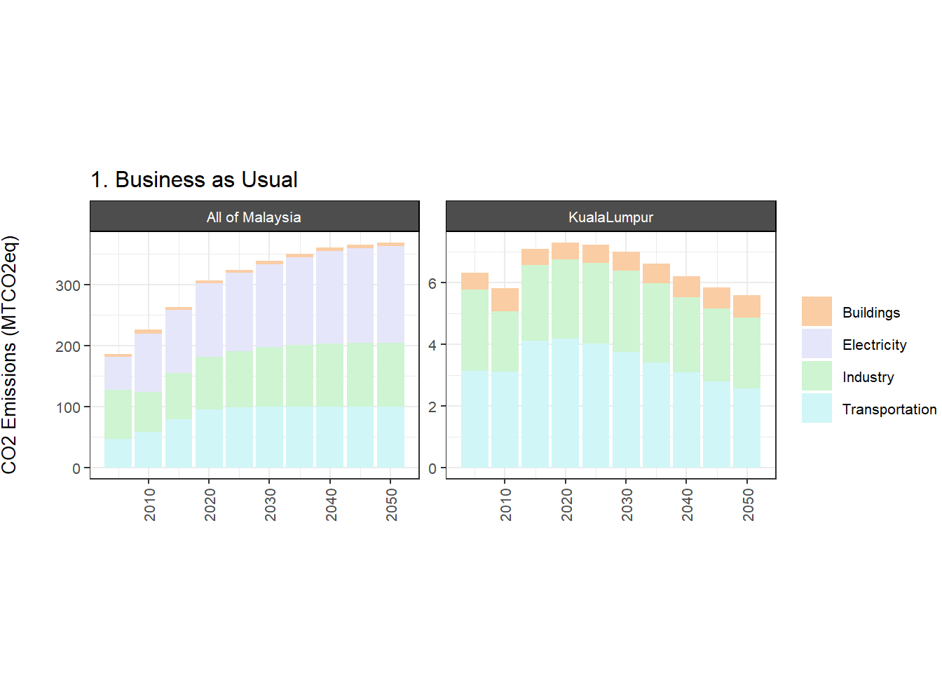
7.2.1.2 Emissions by Sector and Gas

7.2.1.2.1 Malaysia and Kuala Lumpur

co2 <- malaysia %>% filter(param == "emissCO2BySectorNoBio",
                           region != "Malaysia") %>%
  mutate(#value = value * 3.67,
         units = "CO2 Emissions (MTCO2eq)")

malaysia_emissions <- co2 %>%
  mutate(class = case_when(grepl("International",class)~"Transportation",
                           grepl("alumin|desalinated|refining|urban|coal|gas|oil|hydrogen|agricultural|crops",class)~"Industry",
                           TRUE~class)) %>%
  filter(class != "LUC")

emissions <- malaysia_emissions %>%
  mutate(param = units) %>%
  rchart::chart(save = F, 
                show = F,
                size_text = 10)

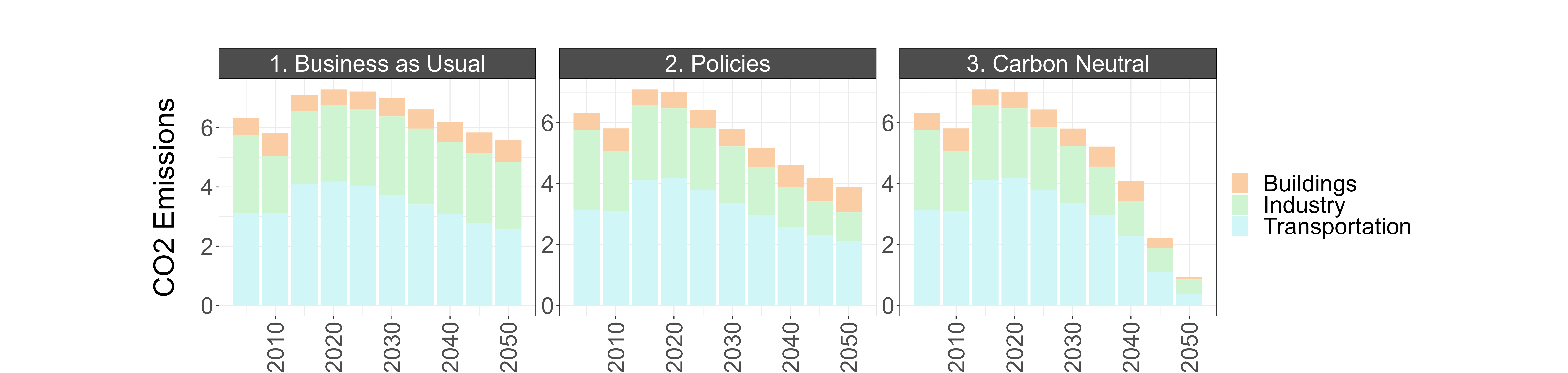
emissions[[c]]

Direct BAU CO₂ emissions by sector in Malaysia and Kuala Lumpur

Direct BAU CO~2~ emissions by sector in Malaysia and Kuala Lumpur

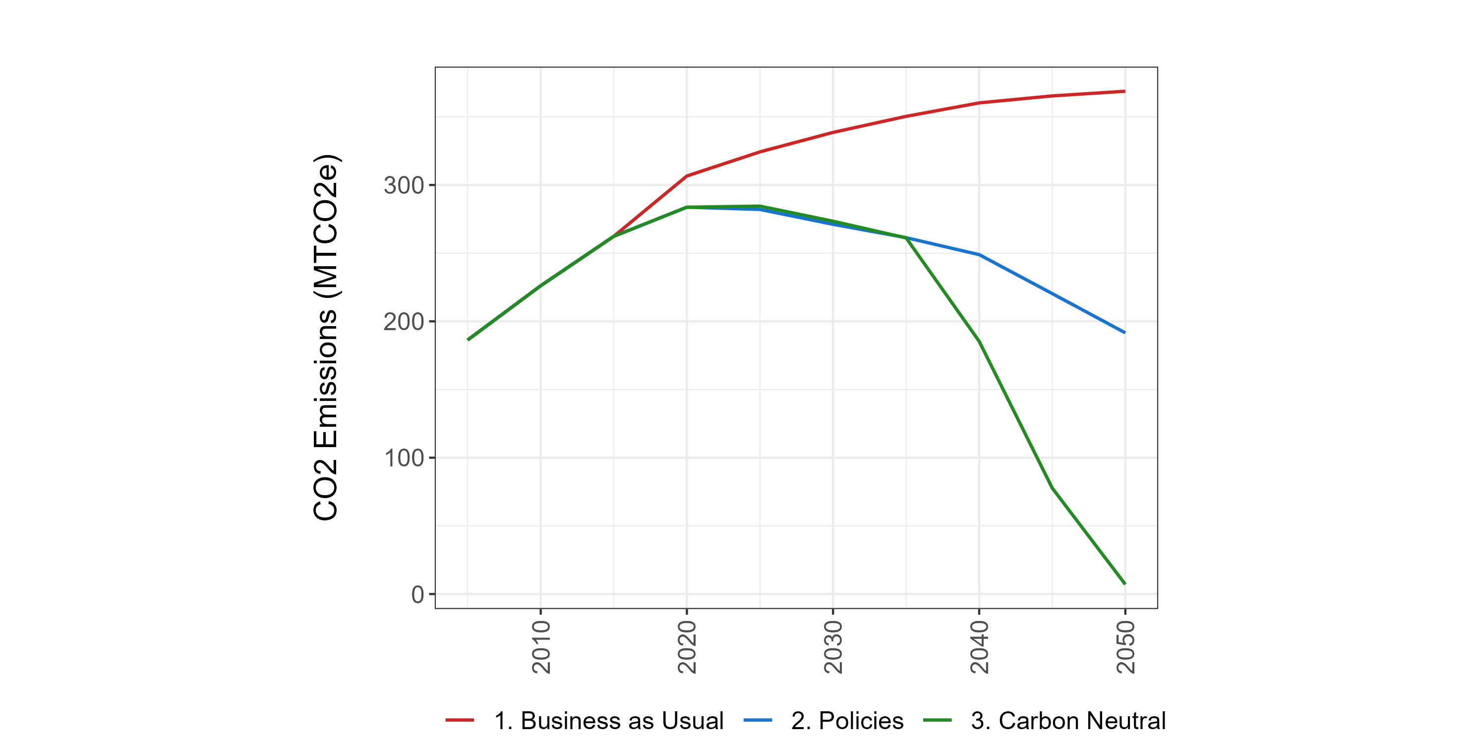
7.2.1.2.2 Malaysia

co2_my <- malaysia %>% 
  filter(param == "emissCO2BySectorNoBio", 
         region == "All of Malaysia",
         class != "LUC") %>%
  mutate(# value = value * 3.67,
         units = "CO2 Emissions (MTCO2e)",
         param = "CO2 Emissions",
         class = case_when(grepl("International",class)~"transport",
                           grepl("refin|hydrogen",class)~"Industry",
                           TRUE~class)) %>% 
  group_by(scenario, region, class, units, param, x, xLabel, classLabel, subRegion, vintage) %>% 
  summarize(value = sum(value)) %>% 
  ungroup() %>%
  mutate(param = units)

emissions_my_plot <- co2_my %>%
  rchart::chart(save = T, 
                show = F,
                scenRef = REF_SCENARIO,
                chart_type = "param_absolute",
                folder = figure_path,
                append = "_co2_lines")

gas_my <- co2_my %>%
  rchart::chart(save = T, 
                show = F,
                chart_type = c("class_absolute", "class_diff_absolute"),
                scenRef = REF_SCENARIO,
                ncol = 4,
                folder = figure_path,
                append = "_co2_emiss",
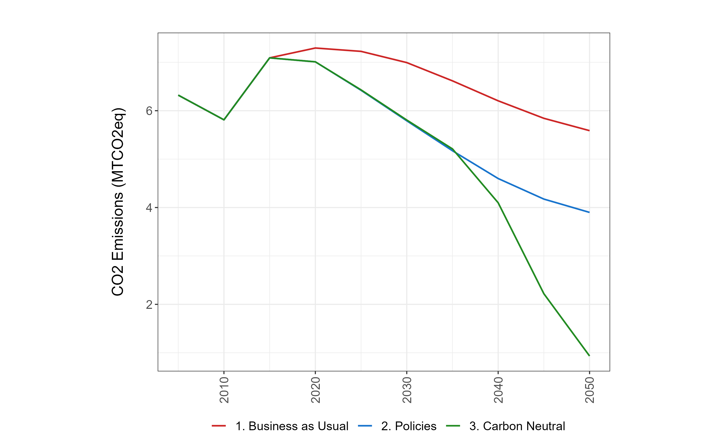
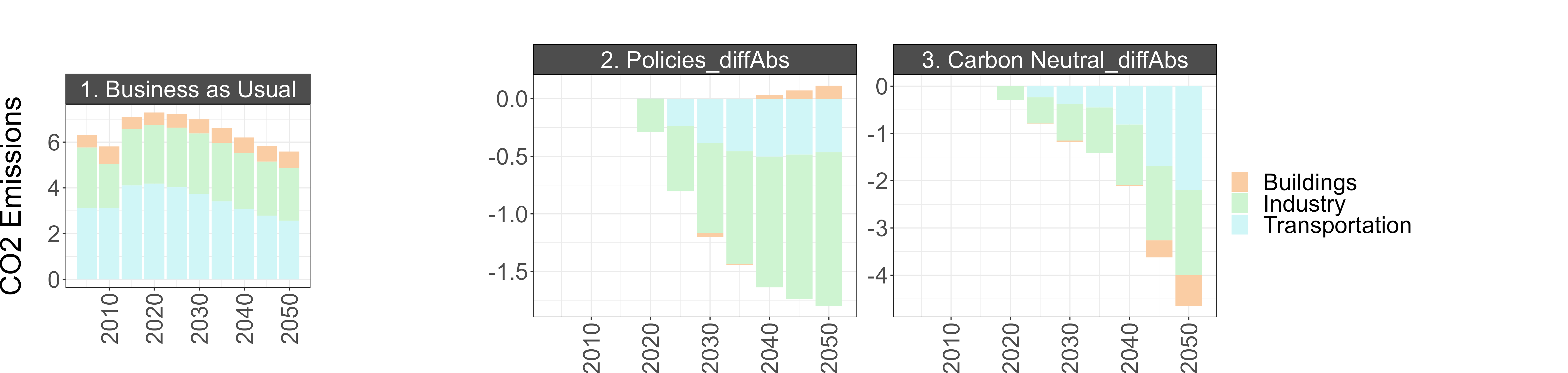
                size_text = 28)

knitr::include_graphics("./markdown_figs/chart_param_co2_lines.png")

Total CO₂ emissions by scenario in Malaysia

Total CO~2~ emissions by scenario in Malaysia

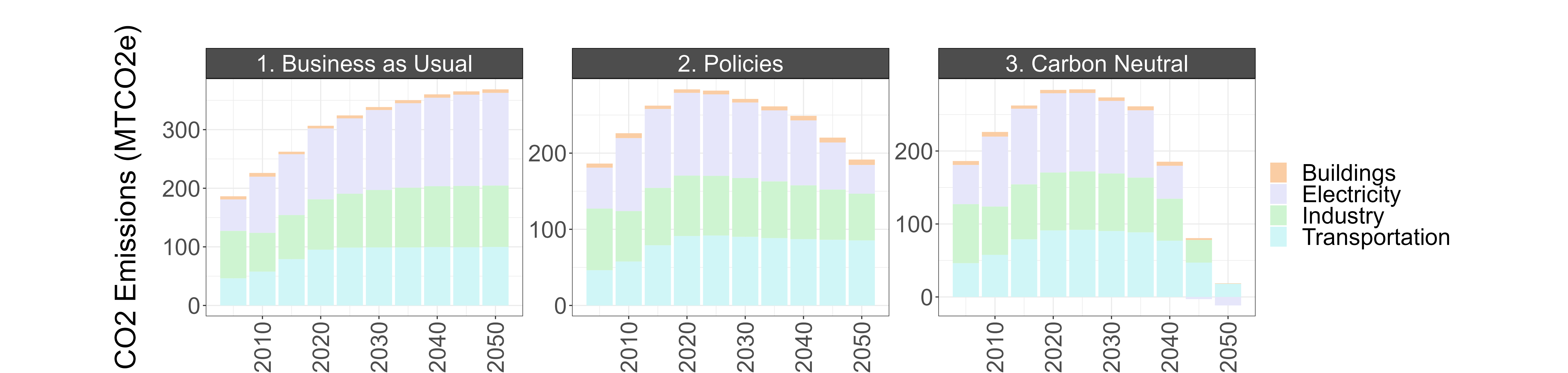
knitr::include_graphics("./markdown_figs/chart_class_co2_emiss.png")

CO₂ emissions by sector in Malaysia

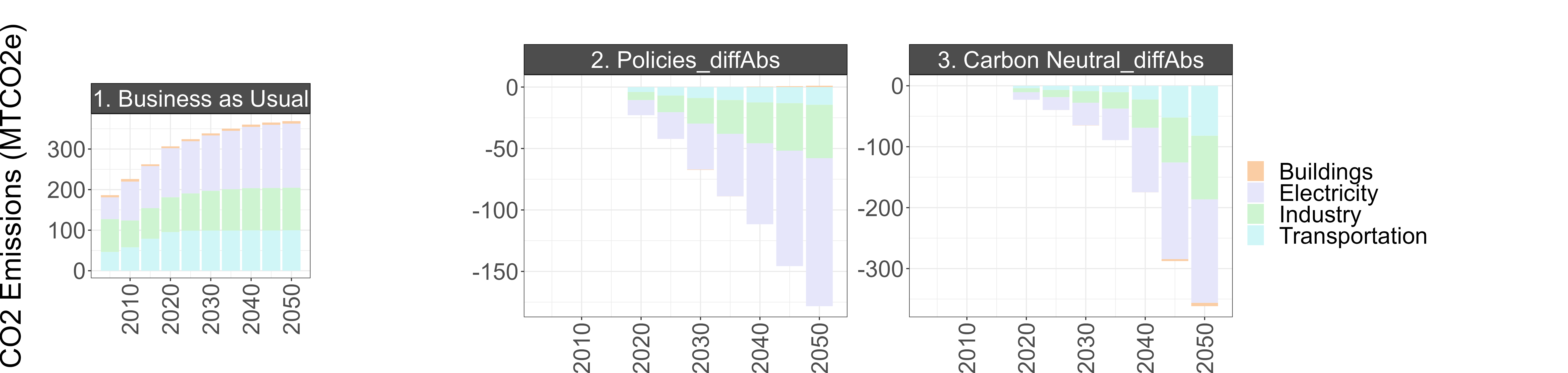
knitr::include_graphics("./markdown_figs/chart_class_diff_absolute_co2_emiss.png")

BAU CO₂ emissions (left) and the difference between BAU and the Policies and Carbon Neutral scenarios

BAU CO~2~ emissions (left) and the difference between BAU and the Policies and Carbon Neutral scenarios

7.2.1.2.3 Kuala Lumpur

co2_kl <- malaysia %>% 
  filter(param == "emissCO2BySectorNoBio",
         region == "KualaLumpur") %>%
  mutate(#value = value * 3.67,
         units = "CO2 Emissions (MTCO2eq)",
         param = "CO2 Emissions",
         class = case_when(grepl("International",class)~"transport", TRUE~class))  %>% 
  group_by(scenario, region, class, units, param, x, xLabel, classLabel, subRegion, vintage) %>% 
  summarize(value = sum(value)) %>% 
  ungroup()

emissions_kl_plot <- co2_kl %>%
  mutate(param = units) %>%
  rchart::chart(save = T, 
                show = F,
                scenRef = REF_SCENARIO,
                chart_type = "param_absolute",
                folder = figure_path,
                append = "_co2_lines_kl")

gas_kl <- co2_kl %>%
  rchart::chart(save = T, 
                show = F,
                chart_type = c("class_absolute", "class_diff_absolute"),
                scenRef = REF_SCENARIO,
                ncol = 4,
                folder = figure_path,
                append = "_co2_emiss_kl",
                size_text = 28)

knitr::include_graphics("./markdown_figs/chart_param_co2_lines_kl.png")

Total CO₂ emissions by scenario in Kuala Lumpur

Total CO~2~ emissions by scenario in Kuala Lumpur

knitr::include_graphics("./markdown_figs/chart_class_co2_emiss_kl.png")

CO₂ emissions by sector in Kuala Lumpur

CO~2~ emissions by sector in Kuala Lumpur

knitr::include_graphics("./markdown_figs/chart_class_diff_absolute_co2_emiss_kl.png")

BAU CO₂ emissions (left) and the difference between BAU and the Policies and Carbon Neutral scenarios

7.2.1.3 Final Energy by Fuel and Sector

7.2.1.3.1 Malaysia

energy_parameters <- c("energyFinalConsumBySecEJ", "energyFinalByFuelEJ")

energy_consum_my <- malaysia %>% 
  filter(param == "energyFinalConsumBySecEJ",
         region == "All of Malaysia") %>%
  mutate(param = units) %>%
  rchart::chart(save = T, 
                show = F,
                chart_type = c("class_absolute", "class_diff_absolute"),
                scenRef = REF_SCENARIO,
                ncol = 4,
                folder = figure_path,
                append = "_energy_consum",
                size_text = 28)

energy_fuel_my <- malaysia %>% 
  filter(param == "energyFinalByFuelEJ",
         region == "All of Malaysia") %>%
  mutate(param = units) %>%
  rchart::chart(save = T, 
                show = F,
                chart_type = c("class_absolute", "class_diff_absolute"),
                scenRef = REF_SCENARIO,
                ncol = 4,
                folder = figure_path,
                append = "_energy_fuel",
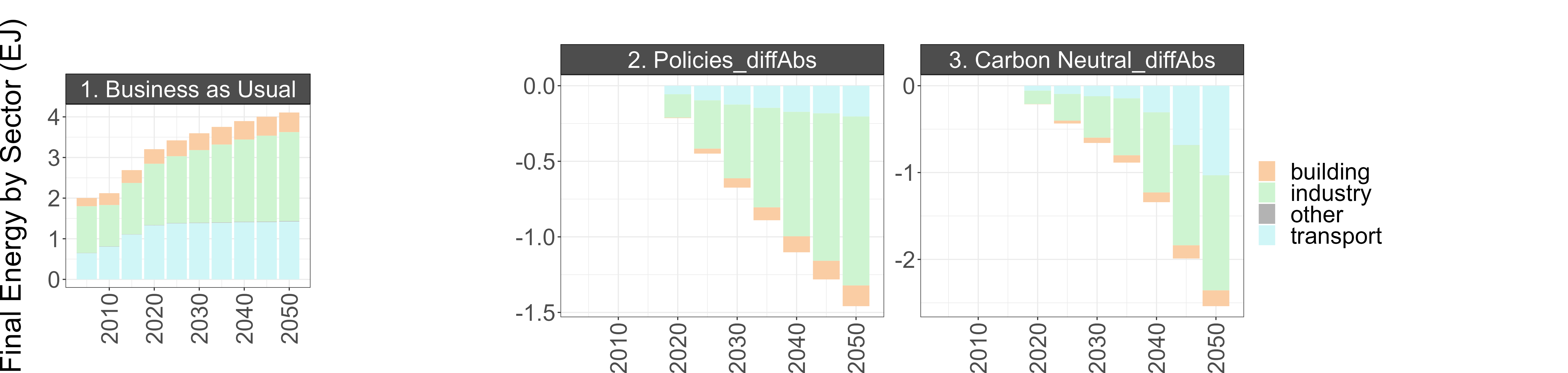
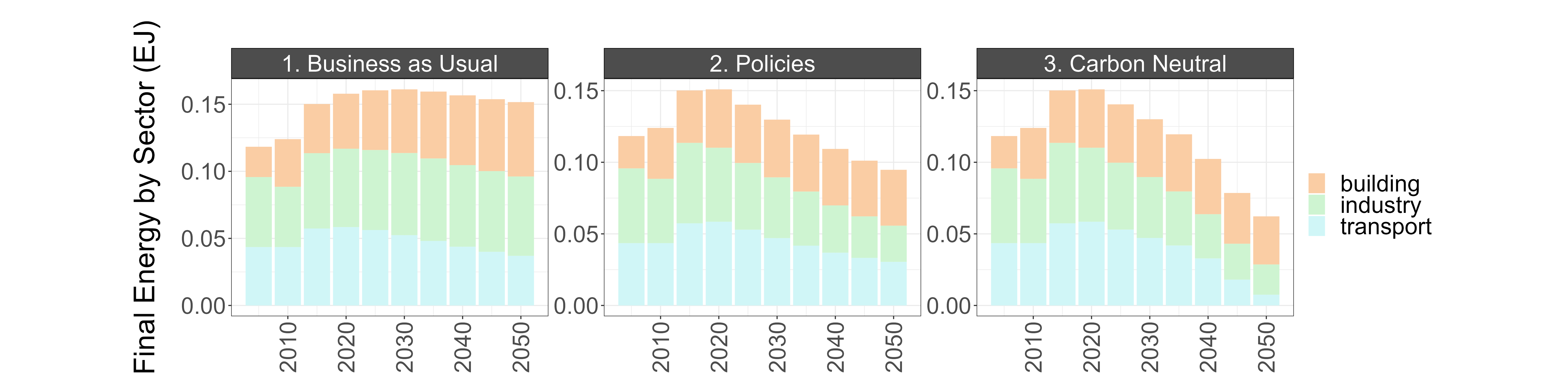
                size_text = 30)

knitr::include_graphics("./markdown_figs/chart_class_energy_consum.png")

Energy consumption by sector in Malaysia

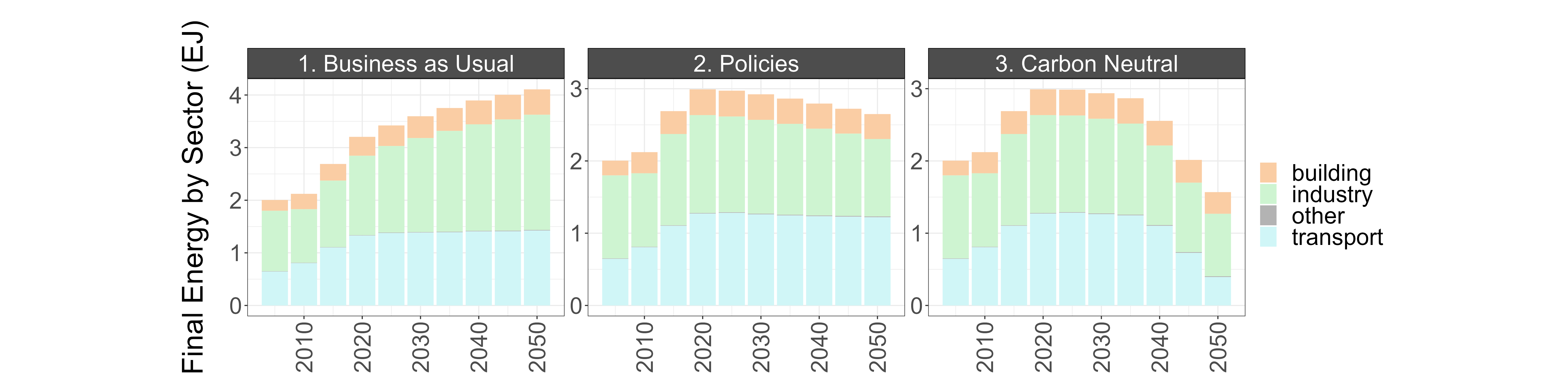
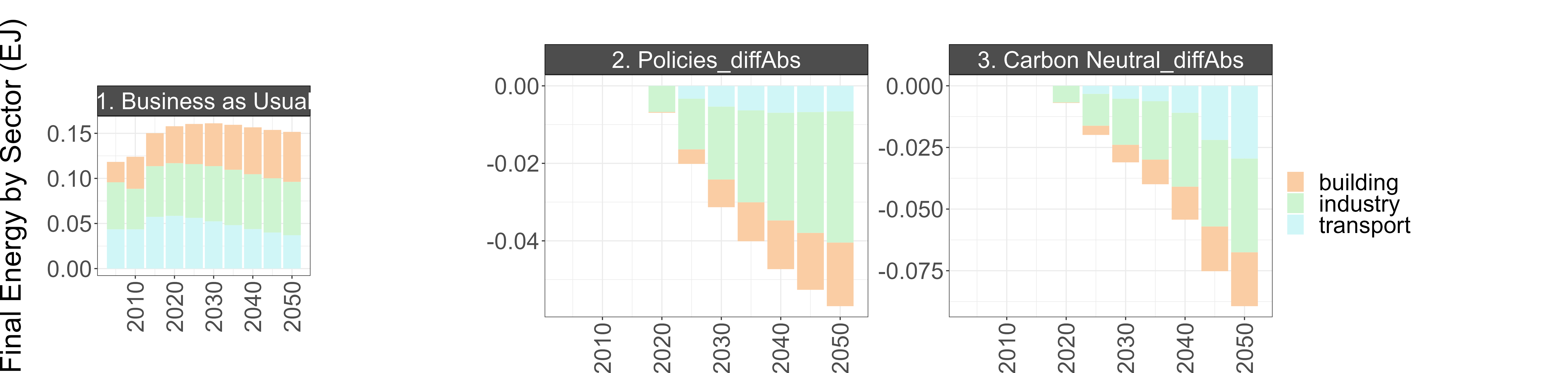
knitr::include_graphics("./markdown_figs/chart_class_diff_absolute_energy_consum.png")

BAU energy consumption (left) and the difference between BAU and the Policies and Carbon Neutral scenarios

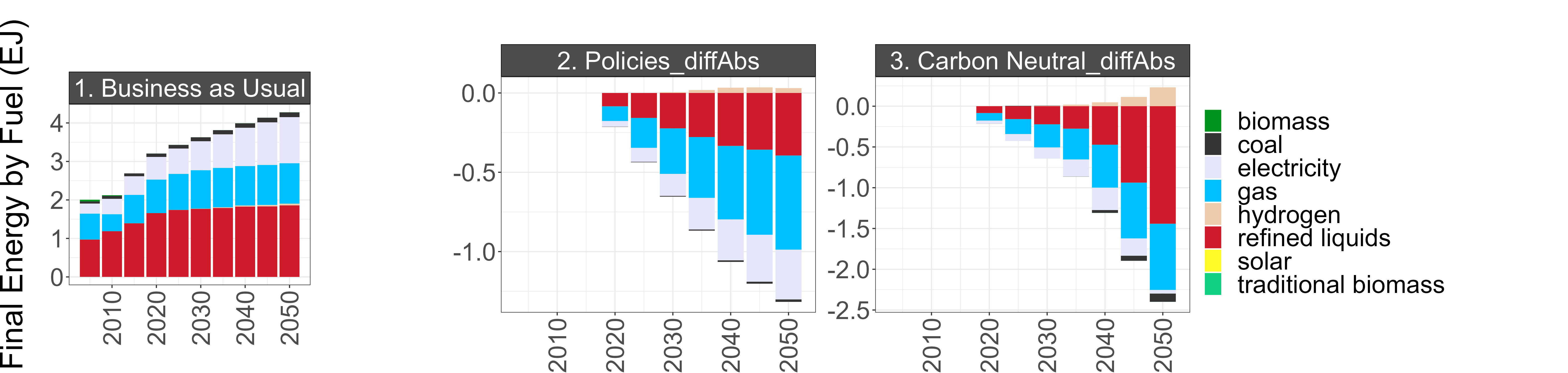
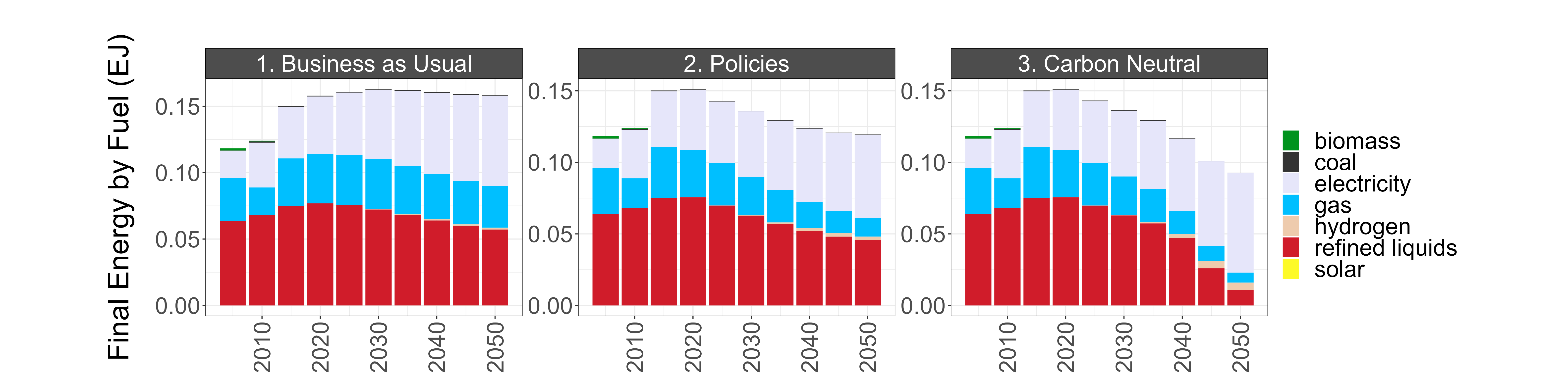
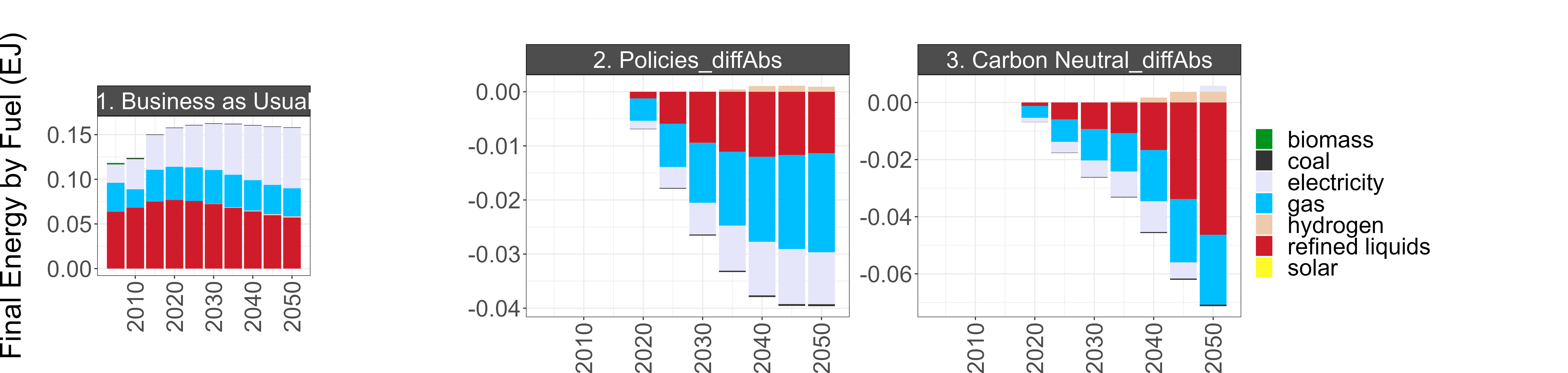
knitr::include_graphics("./markdown_figs/chart_class_energy_fuel.png")

Energy consumption by fuel in Malaysia

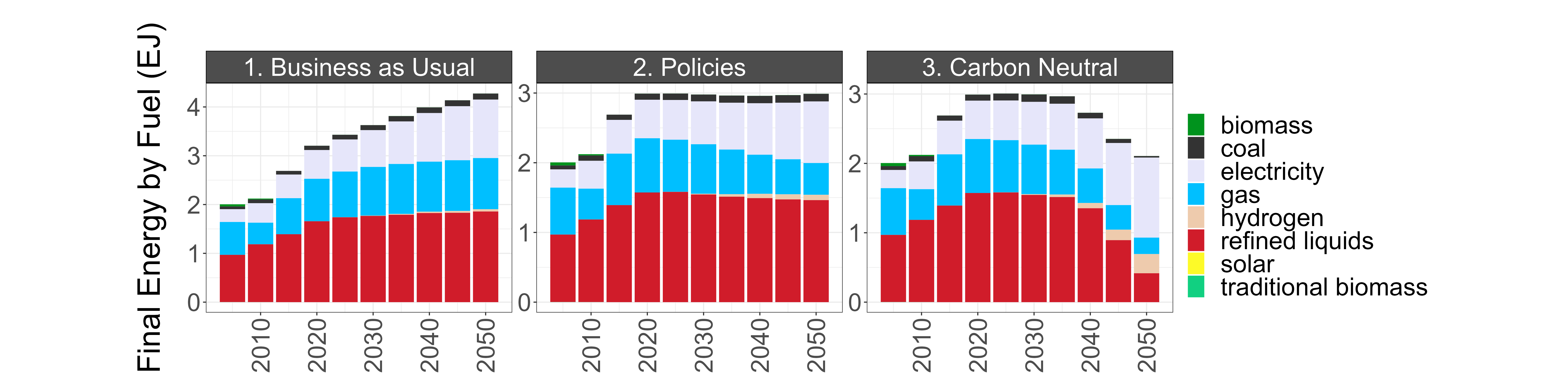
knitr::include_graphics("./markdown_figs/chart_class_diff_absolute_energy_fuel.png")

BAU energy consumption (left) and the difference between BAU and the Policies and Carbon Neutral scenarios

7.2.1.3.2 Kuala Lumpur

energy_kl <- malaysia %>% 
  filter(param == "energyFinalConsumBySecEJ",
         region == "KualaLumpur") %>%
  mutate(param = units) %>%
  rchart::chart(save = T, 
                show = F,
                chart_type = c("class_absolute", "class_diff_absolute"),
                scenRef = REF_SCENARIO,
                ncol = 4,
                folder = figure_path,
                append = "_energy_consum_kl",
                size_text = 28)

energy_kl <- malaysia %>% 
  filter(param == "energyFinalByFuelEJ",
         region == "KualaLumpur") %>%
  mutate(param = units) %>%
  rchart::chart(save = T, 
                show = F,
                chart_type = c("class_absolute", "class_diff_absolute"),
                scenRef = REF_SCENARIO,
                ncol = 4,
                folder = figure_path,
                append = "_energy_fuel_kl",
                size_text = 28)

knitr::include_graphics("./markdown_figs/chart_class_energy_consum_kl.png")

Energy consumption by sector in Kuala Lumpur

knitr::include_graphics("./markdown_figs/chart_class_diff_absolute_energy_consum_kl.png")

BAU energy consumption (left) and the difference between BAU and the Policies and Carbon Neutral scenarios

knitr::include_graphics("./markdown_figs/chart_class_energy_fuel_kl.png")

Energy consumption by fuel in Kuala Lumpur

knitr::include_graphics("./markdown_figs/chart_class_diff_absolute_energy_fuel_kl.png")

BAU energy consumption (left) and the difference between BAU and the Policies and Carbon Neutral scenarios

7.2.1.4 Electricity Generation by Fuel

electricity_my <- malaysia %>% 
  filter(param == "elecByTechTWh",
         region == "All of Malaysia") %>%
  mutate(param = "Electricity Generation\nby Fuel (TWh)") %>%
  rchart::chart(save = T, 
                show = F,
                chart_type = c("class_absolute", "class_diff_absolute"),
                scenRef = REF_SCENARIO,
                ncol = 4,
                folder = figure_path,
                append = "_elec_gen",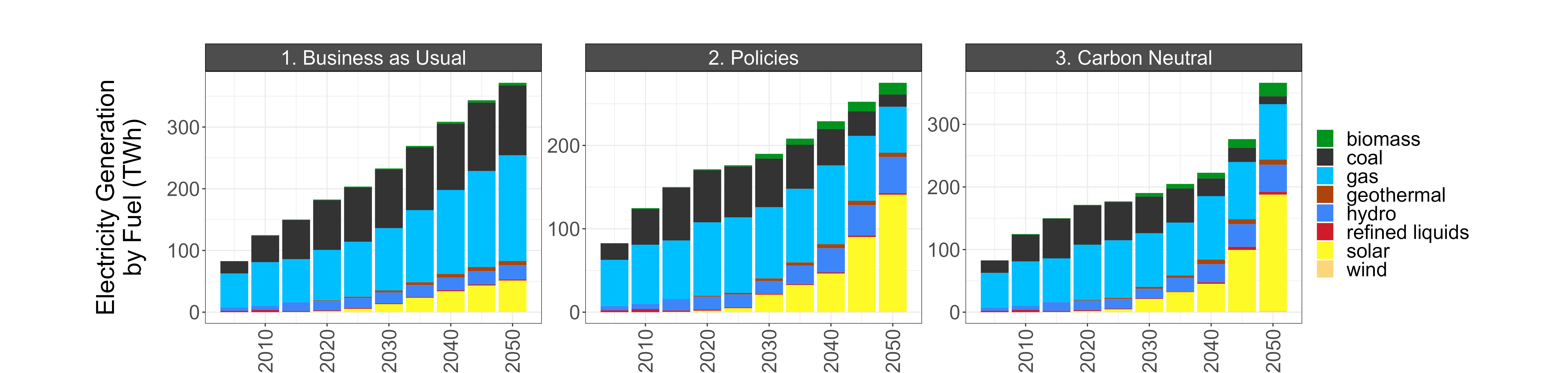
                size_text = 24)

knitr::include_graphics("./markdown_figs/chart_class_elec_gen.png")

Electricity generation by fuel in Malaysia

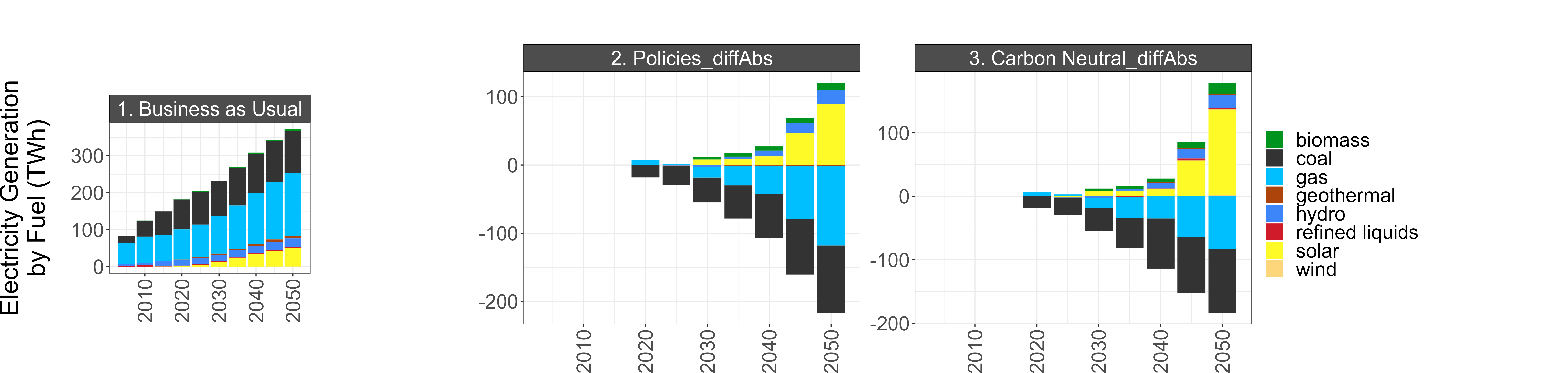
knitr::include_graphics("./markdown_figs/chart_class_diff_absolute_elec_gen.png")

BAU electricity generation (left) and the difference between BAU and the Policies and Carbon Neutral scenarios

7.2.2 Sectoral Details

7.2.2.1 Building Energy by Subsector

7.2.2.1.1 Malaysia

building_energy_resid_my <- malaysia %>% 
  filter(param == "energyFinalSubsecByResidSectorBuildEJ",
         region == "All of Malaysia") %>%
  mutate(param = "Final Energy (EJ)") %>%
  rchart::chart(save = T, 
                show = F,
                chart_type = c("class_absolute", "class_diff_absolute"),
                scenRef = REF_SCENARIO,
                ncol = 4,
                folder = figure_path,
                append = "_resid_bld",
                size_text = 24)

building_energy_comm_my <- malaysia %>% 
  filter(param == "energyFinalSubsecByCommSectorBuildEJ",
         region == "All of Malaysia") %>%
  mutate(param = "Final Energy (EJ)") %>%
  rchart::chart(save = T, 
                show = F,
                chart_type = c("class_absolute", "class_diff_absolute"),
                scenRef = REF_SCENARIO,
                ncol = 4,
                folder = figure_path,
                append = "_comm_bld",
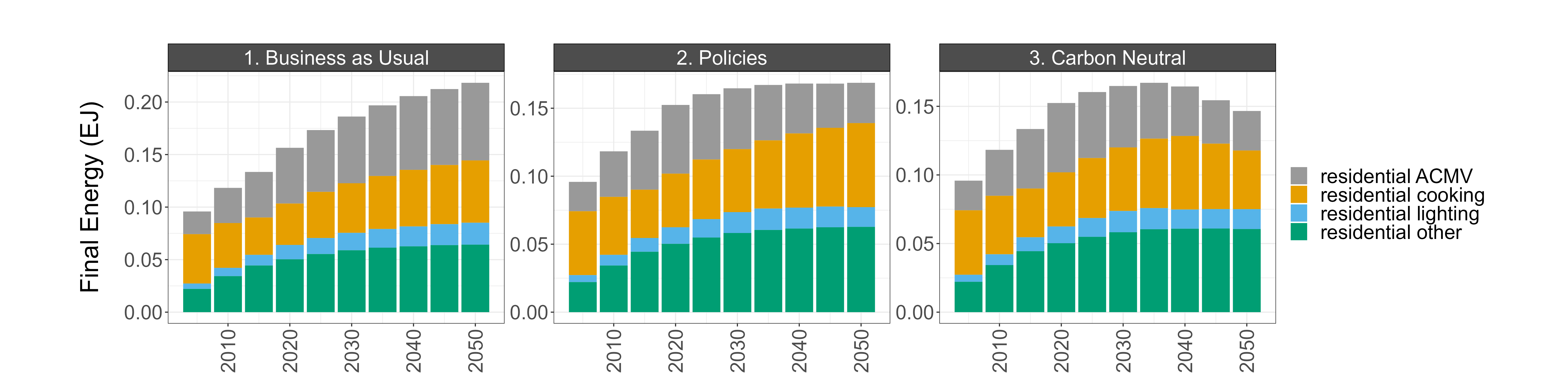
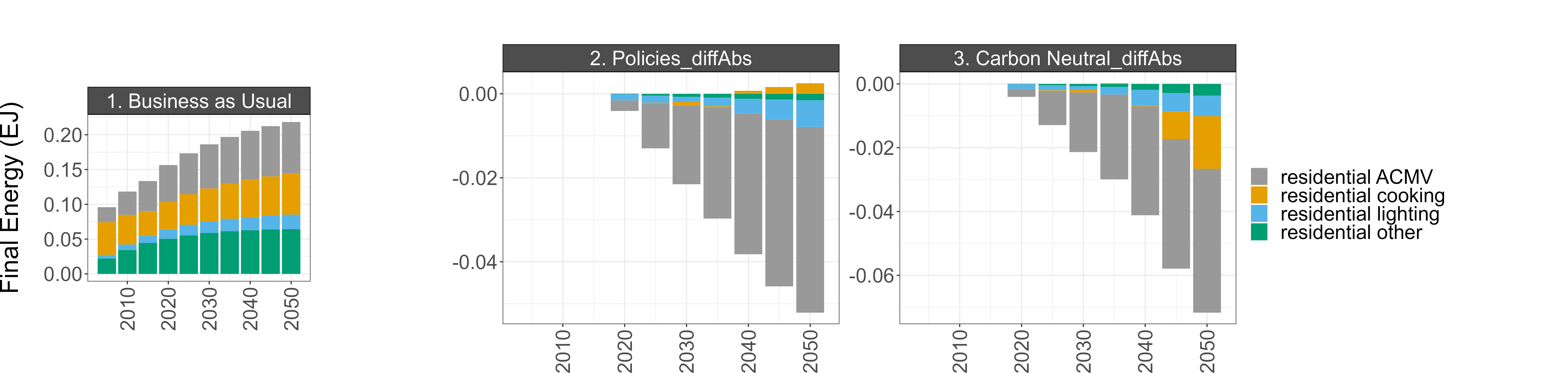
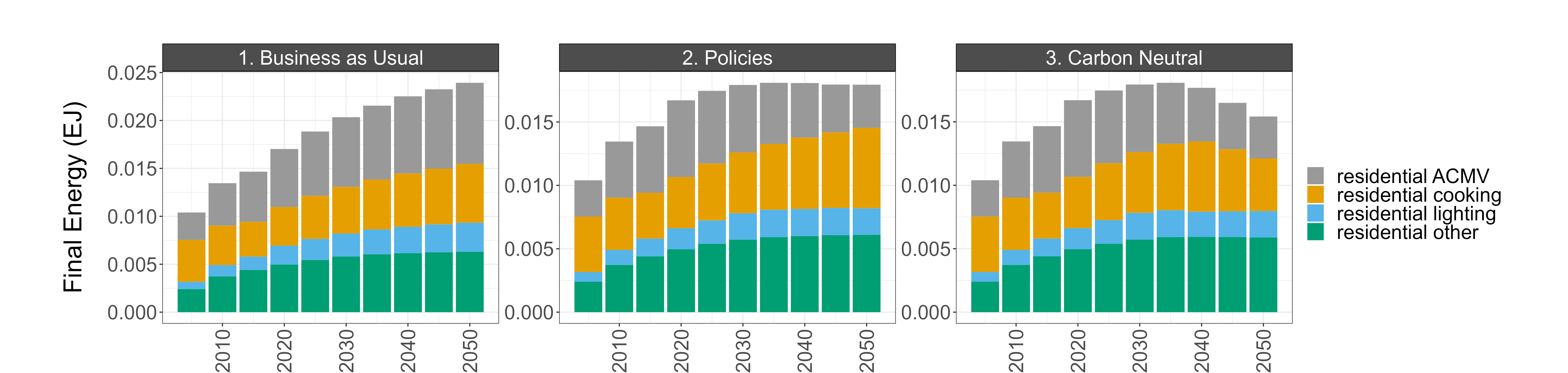
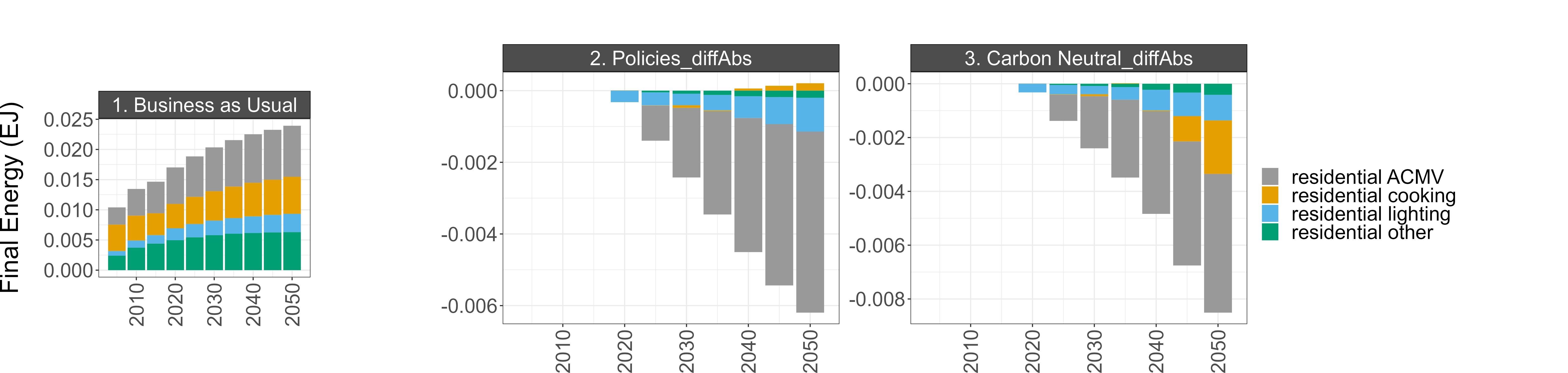
                size_text = 24)

knitr::include_graphics("./markdown_figs/chart_class_resid_bld.png")

Residential building energy consumption by sector in Malaysia

knitr::include_graphics("./markdown_figs/chart_class_diff_absolute_resid_bld.png")

BAU energy consumption (left) and the difference between BAU and the Policies and Carbon Neutral scenarios

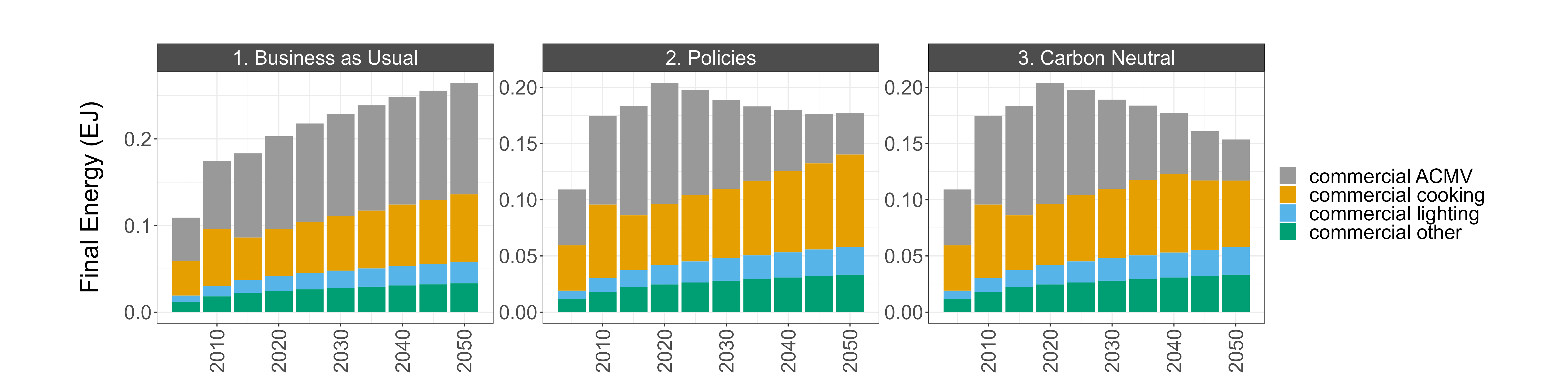
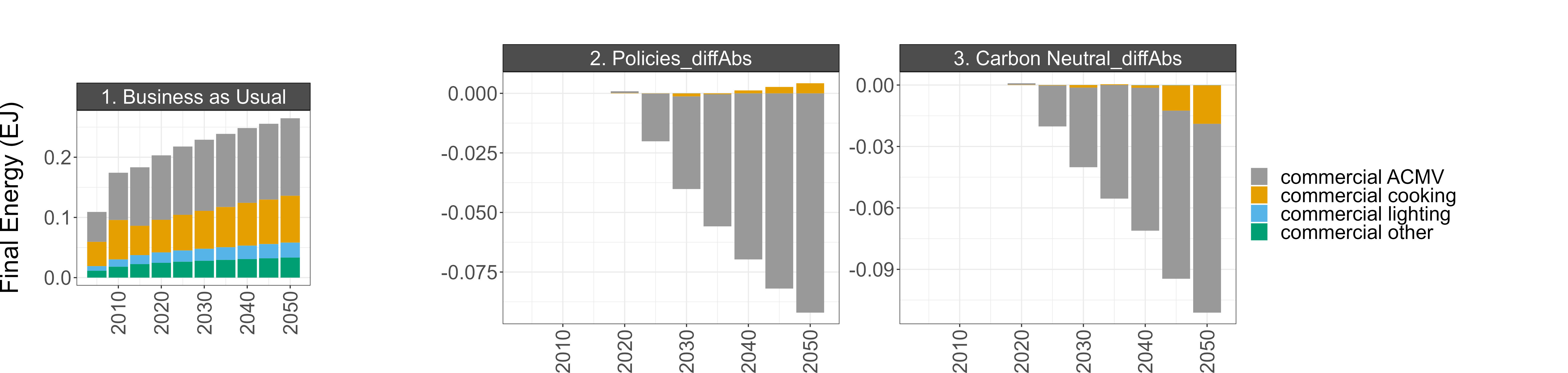
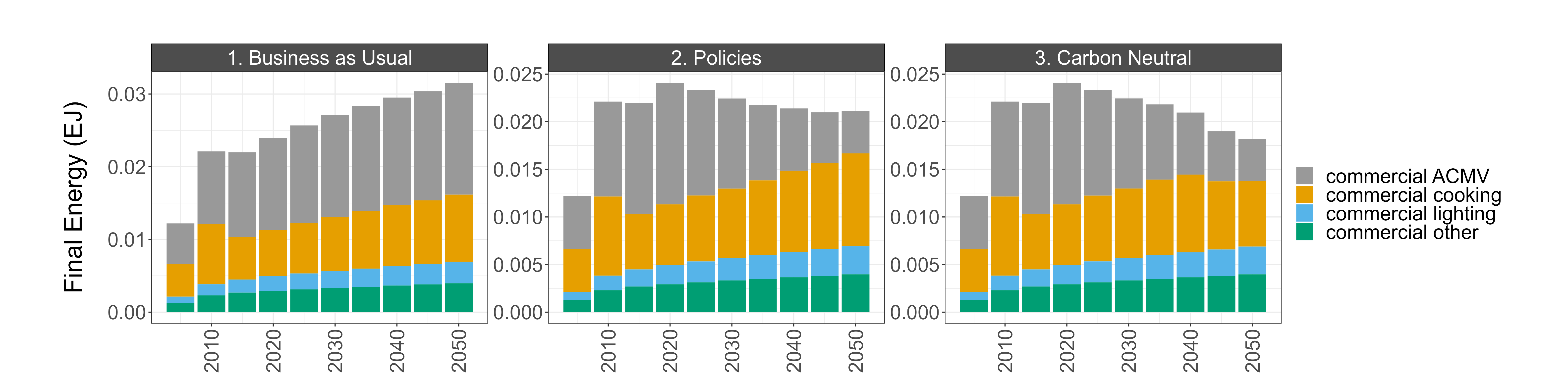
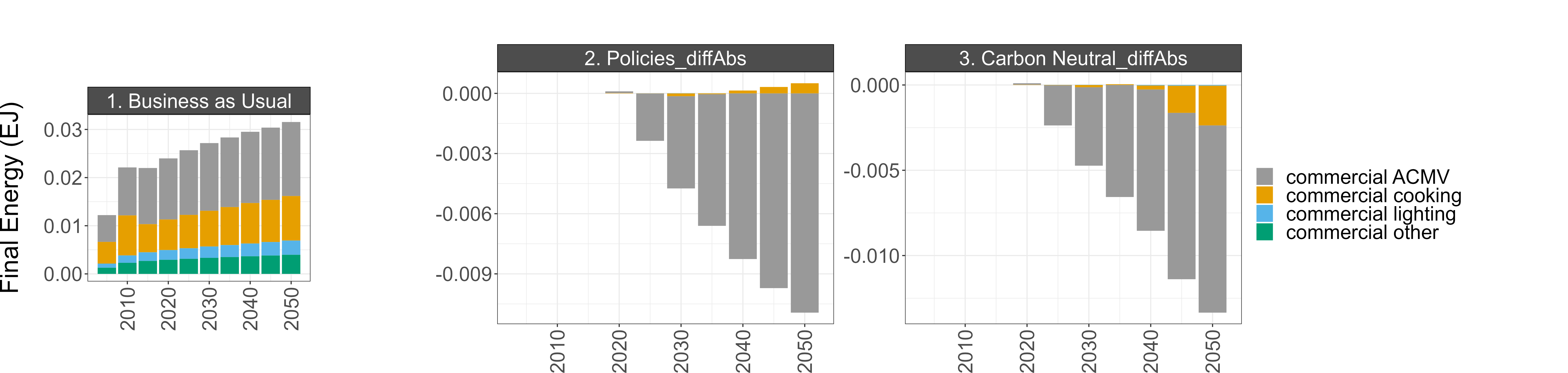
knitr::include_graphics("./markdown_figs/chart_class_comm_bld.png")

Commercial building energy consumption by sector in Malaysia

knitr::include_graphics("./markdown_figs/chart_class_diff_absolute_comm_bld.png")

BAU energy consumption (left) and the difference between BAU and the Policies and Carbon Neutral scenarios

7.2.2.1.2 Kuala Lumpur

building_energy_resid_kl <- malaysia %>% 
  filter(param == "energyFinalSubsecByResidSectorBuildEJ",
         region == "KualaLumpur") %>%
  mutate(param = "Final Energy (EJ)") %>%
  rchart::chart(save = T, 
                show = F,
                chart_type = c("class_absolute", "class_diff_absolute"),
                scenRef = REF_SCENARIO,
                ncol = 4,
                folder = figure_path,
                append = "_resid_bld_kl",
                size_text = 24)

building_energy_comm_kl <- malaysia %>% 
  filter(param == "energyFinalSubsecByCommSectorBuildEJ",
         region == "KualaLumpur") %>%
  mutate(param = "Final Energy (EJ)") %>%
  rchart::chart(save = T, 
                show = F,
                chart_type = c("class_absolute", "class_diff_absolute"),
                scenRef = REF_SCENARIO,
                ncol = 4,
                folder = figure_path,
                append = "_comm_bld_kl",
                size_text = 24)

knitr::include_graphics("./markdown_figs/chart_class_resid_bld_kl.png")

Residential building energy consumption by sector in Kuala Lumpur

knitr::include_graphics("./markdown_figs/chart_class_diff_absolute_resid_bld_kl.png")

BAU energy consumption (left) and the difference between BAU and the Policies and Carbon Neutral scenarios

knitr::include_graphics("./markdown_figs/chart_class_comm_bld_kl.png")

Commercial building energy consumption by sector in Kuala Lumpur

knitr::include_graphics("./markdown_figs/chart_class_diff_absolute_comm_bld_kl.png")

BAU energy consumption (left) and the difference between BAU and the Policies and Carbon Neutral scenarios

7.2.2.2 Transportation by Mode

7.2.2.2.1 Malaysia

transport_my_m <- malaysia %>% 
  filter(param == "transportFreightVMTByMode",
         region == "All of Malaysia") %>%
  mutate(param = units) %>%
  rchart::chart(save = T, 
                show = F,
                chart_type = c("class_absolute", "class_diff_absolute"),
                scenRef = REF_SCENARIO,
                ncol = 4,
                folder = figure_path,
                append = "_freight_mode",
                size_text = 24)

transport_my_m <- malaysia %>% 
  filter(param == "transportPassengerVMTByMode",
         region == "All of Malaysia") %>%
  mutate(param = units) %>%
  rchart::chart(save = T, 
                show = F,
                chart_type = c("class_absolute", "class_diff_absolute"),
                scenRef = REF_SCENARIO,
                ncol = 4,
                folder = figure_path,
                append = "_pass_mode",
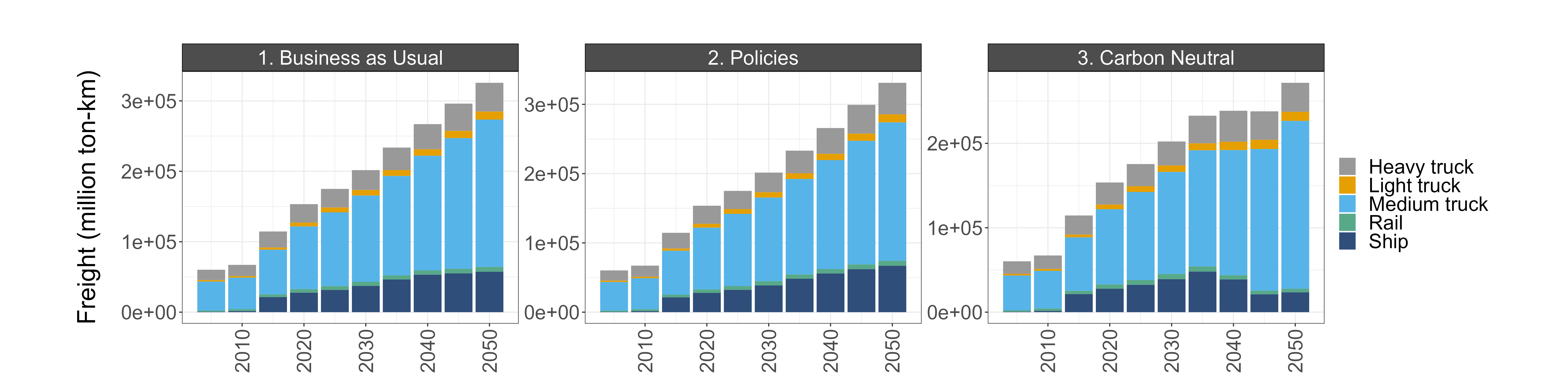
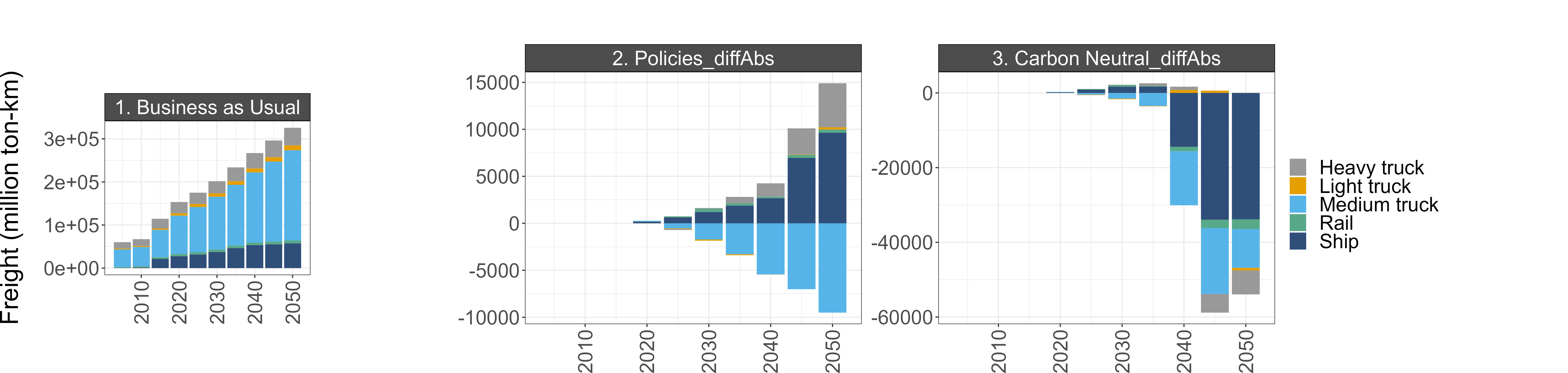
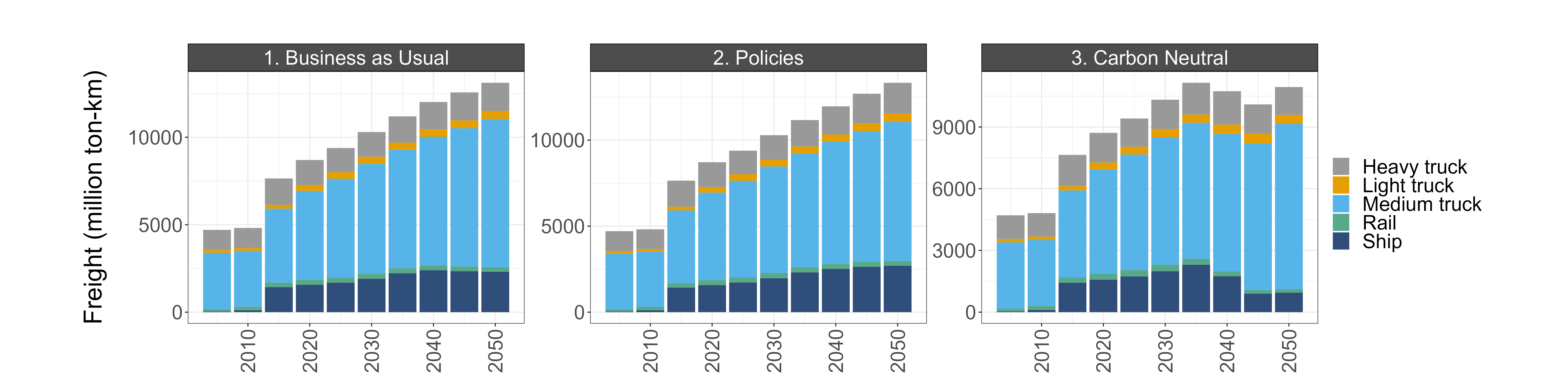
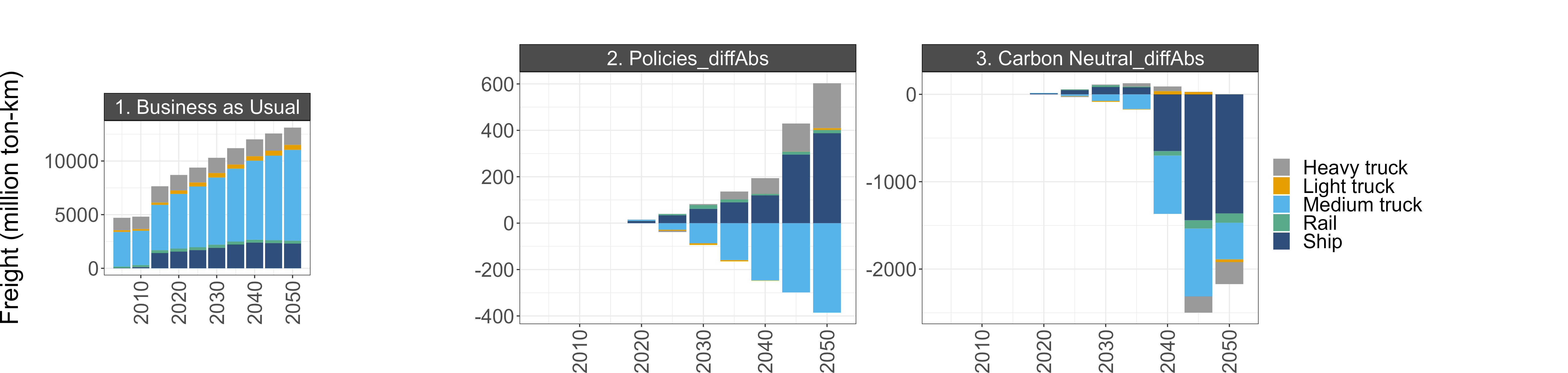
                size_text = 24)

knitr::include_graphics("./markdown_figs/chart_class_freight_mode.png")

Freight vehicle kilometers traveled by mode in Malaysia

knitr::include_graphics("./markdown_figs/chart_class_diff_absolute_freight_mode.png")

BAU freight vehicle kilometers traveled (left) and the difference between BAU and the Policies and Carbon Neutral scenarios

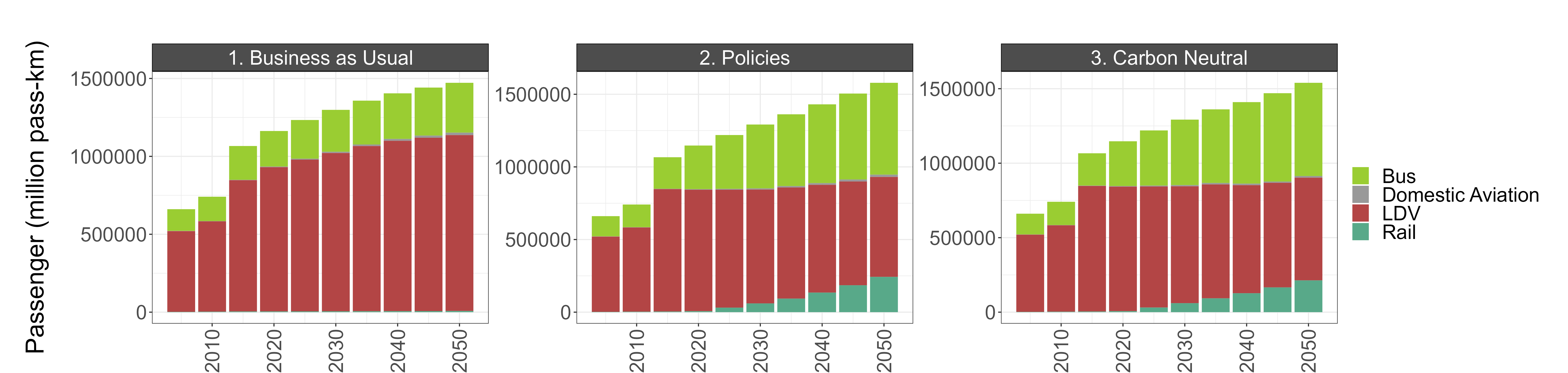
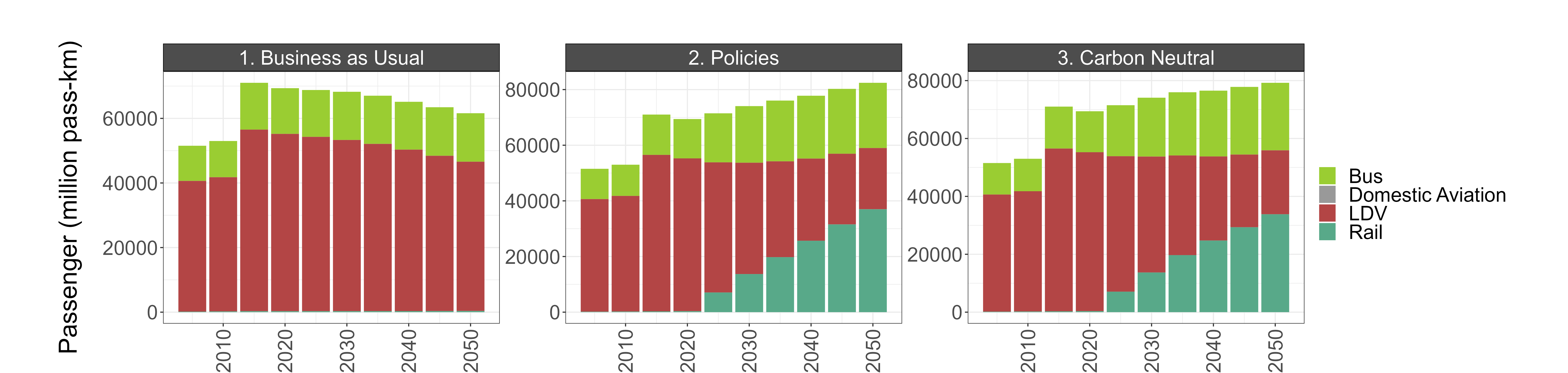
knitr::include_graphics("./markdown_figs/chart_class_pass_mode.png")

Passenger vehicle kilometers traveled by mode in Malaysia

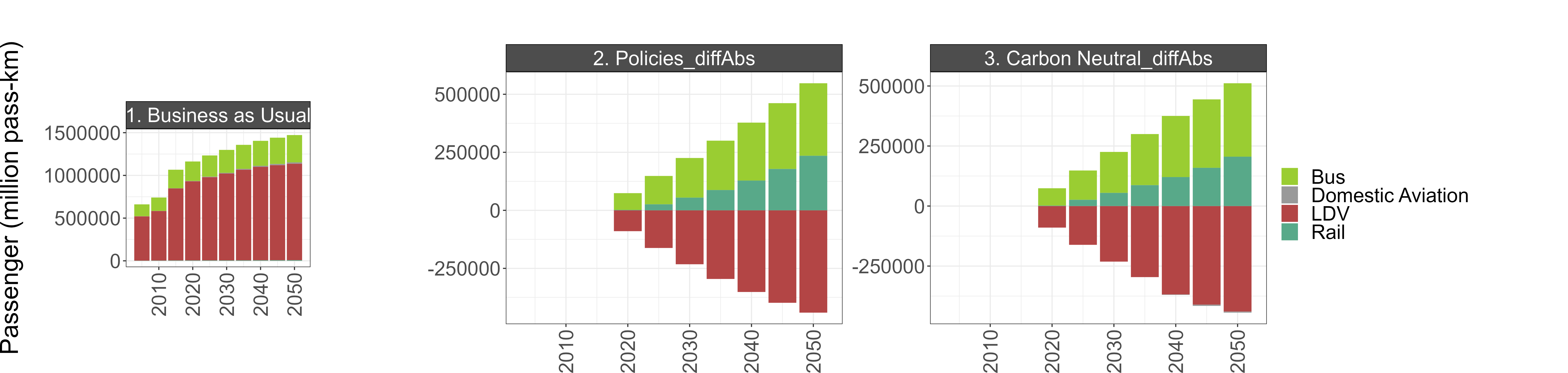
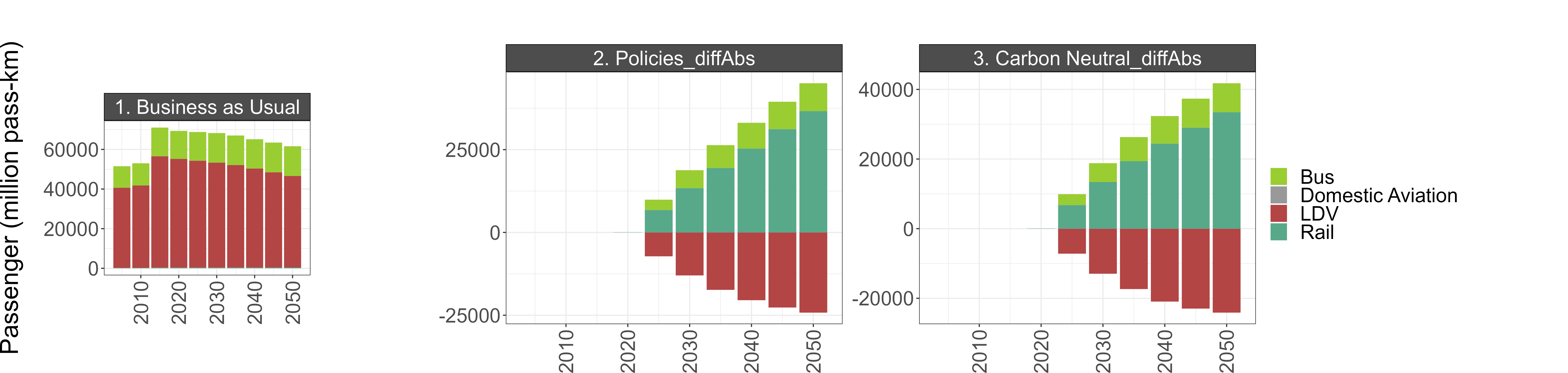
knitr::include_graphics("./markdown_figs/chart_class_diff_absolute_pass_mode.png")

BAU passenger vehicle kilometers traveled (left) and the difference between BAU and the Policies and Carbon Neutral scenarios

7.2.2.2.2 Kuala Lumpur

transport_kl_m <- malaysia %>% 
  filter(param == "transportFreightVMTByMode",
         region == "KualaLumpur") %>%
  mutate(param = units) %>%
  rchart::chart(save = T, 
                show = F,
                chart_type = c("class_absolute", "class_diff_absolute"),
                scenRef = REF_SCENARIO,
                ncol = 4,
                folder = figure_path,
                append = "_freight_mode_kl",
                size_text = 24)

transport_kl_m <- malaysia %>% 
  filter(param == "transportPassengerVMTByMode",
         region == "KualaLumpur") %>%
  mutate(param = units) %>%
  rchart::chart(save = T, 
                show = F,
                chart_type = c("class_absolute", "class_diff_absolute"),
                scenRef = REF_SCENARIO,
                ncol = 4,
                folder = figure_path,
                append = "_pass_mode_kl",
                size_text = 24)

knitr::include_graphics("./markdown_figs/chart_class_freight_mode_kl.png")

Freight vehicle kilometers traveled in Kuala Lumpur

knitr::include_graphics("./markdown_figs/chart_class_diff_absolute_freight_mode_kl.png")

BAU freight vehicle kilometers traveled (left) and the difference between BAU and the Policies and Carbon Neutral scenarios

knitr::include_graphics("./markdown_figs/chart_class_pass_mode_kl.png")

Passenger vehicle kilometers traveled in Kuala Lumpur

knitr::include_graphics("./markdown_figs/chart_class_diff_absolute_pass_mode_kl.png")

BAU passenger vehicle kilometers traveled (left) and the difference between BAU and the Policies and Carbon Neutral scenarios

7.2.2.3 Transportation by Fuel

7.2.2.3.1 Malaysia

transport_my_f <- malaysia %>% 
  filter(param == "energyFinalByFuelTransportFreightEJ",
         region == "All of Malaysia") %>%
  mutate(param = units) %>%
  rchart::chart(save = T, 
                show = F,
                chart_type = c("class_absolute", "class_diff_absolute"),
                scenRef = REF_SCENARIO,
                ncol = 4,
                folder = figure_path,
                append = "_freight_fuel",
                size_text = 24)

transport_my_f <- malaysia %>% 
  filter(param == "energyFinalByFuelTransportPassEJ",
         region == "All of Malaysia") %>%
  mutate(param = units) %>%
  rchart::chart(save = T, 
                show = F,
                chart_type = c("class_absolute", "class_diff_absolute"),
                scenRef = REF_SCENARIO,
                ncol = 4,
                folder = figure_path,
                append = "_pass_fuel",
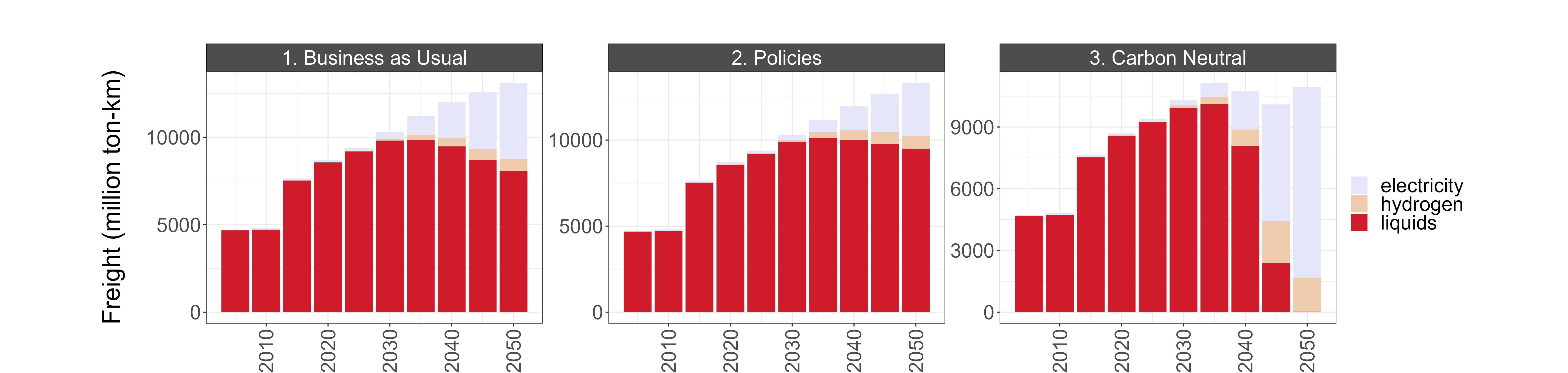
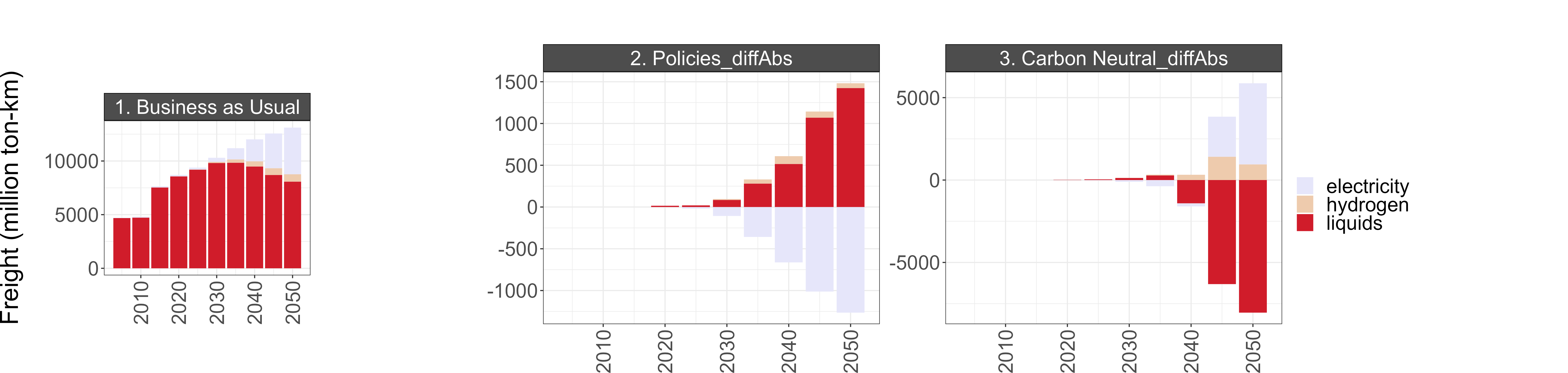
                size_text = 24)

knitr::include_graphics("./markdown_figs/chart_class_freight_fuel.png")

Freight energy consumption by fuel in Malaysia

knitr::include_graphics("./markdown_figs/chart_class_diff_absolute_freight_fuel.png")

BAU energy consumption (left) and the difference between BAU and the Policies and Carbon Neutral scenarios

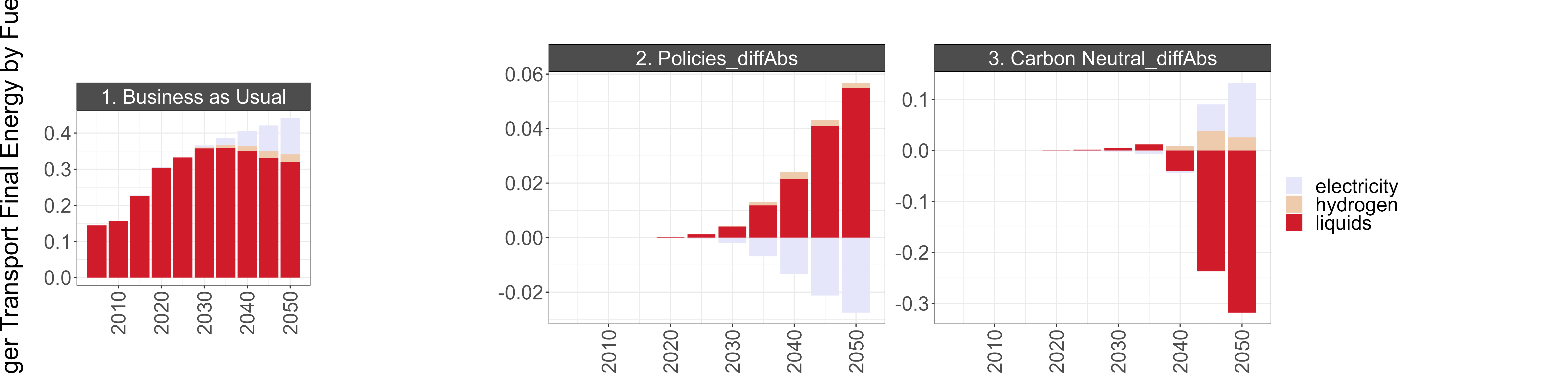
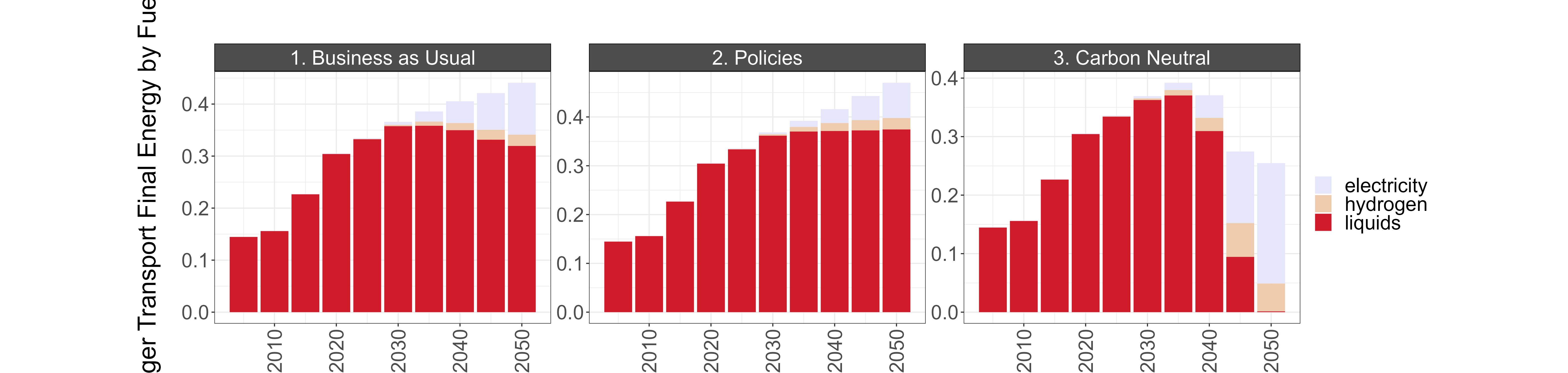
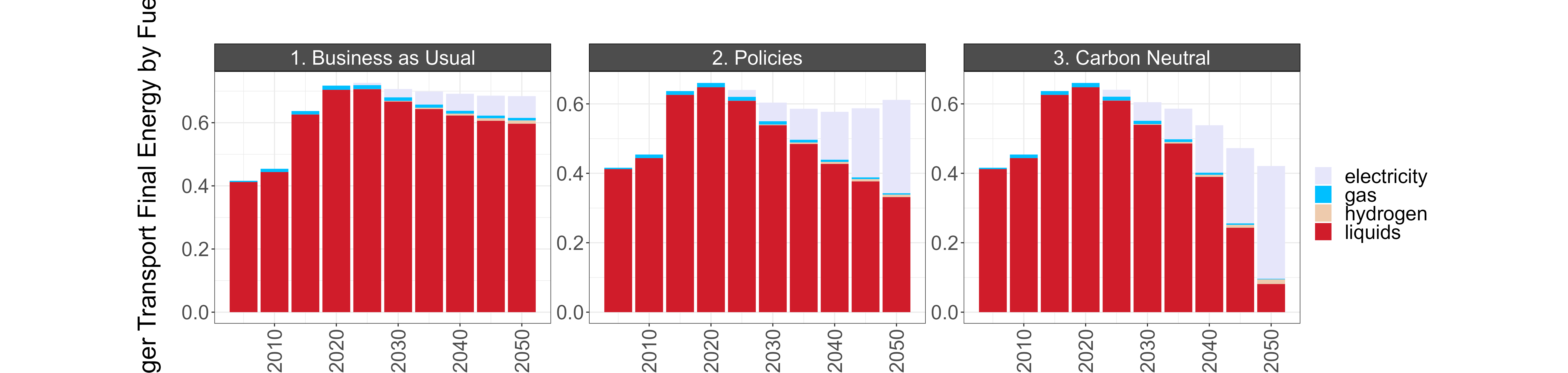
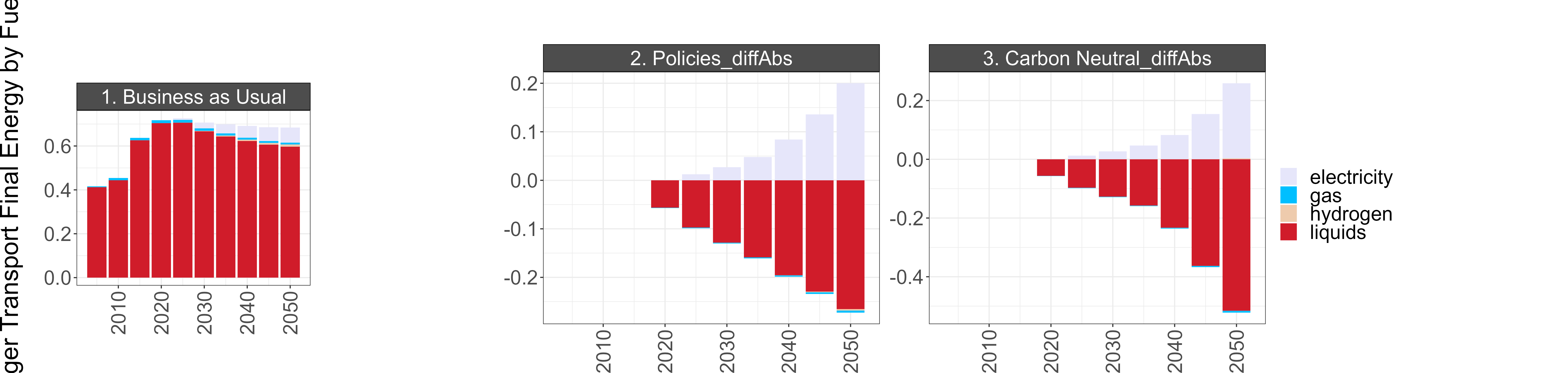
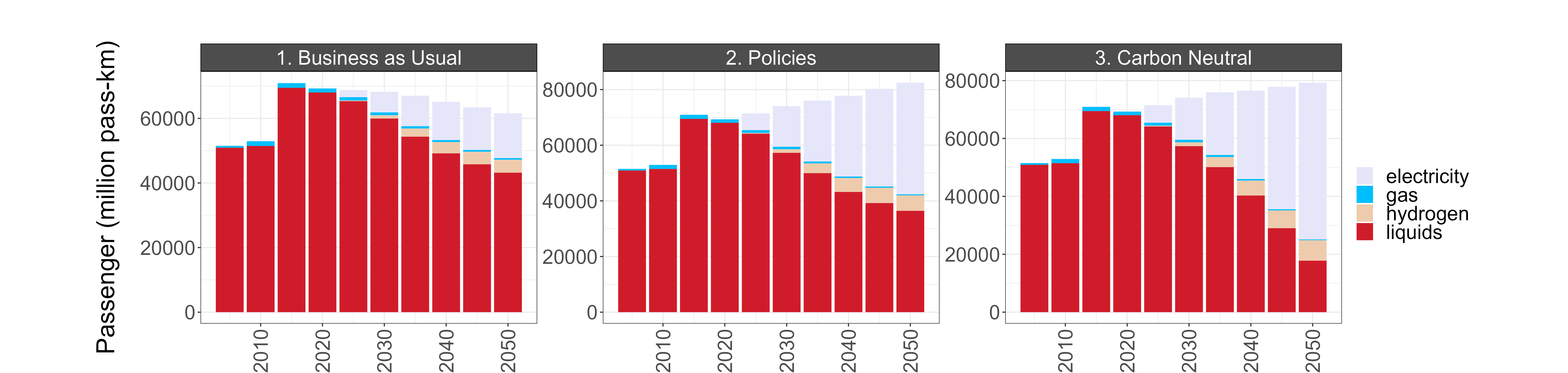
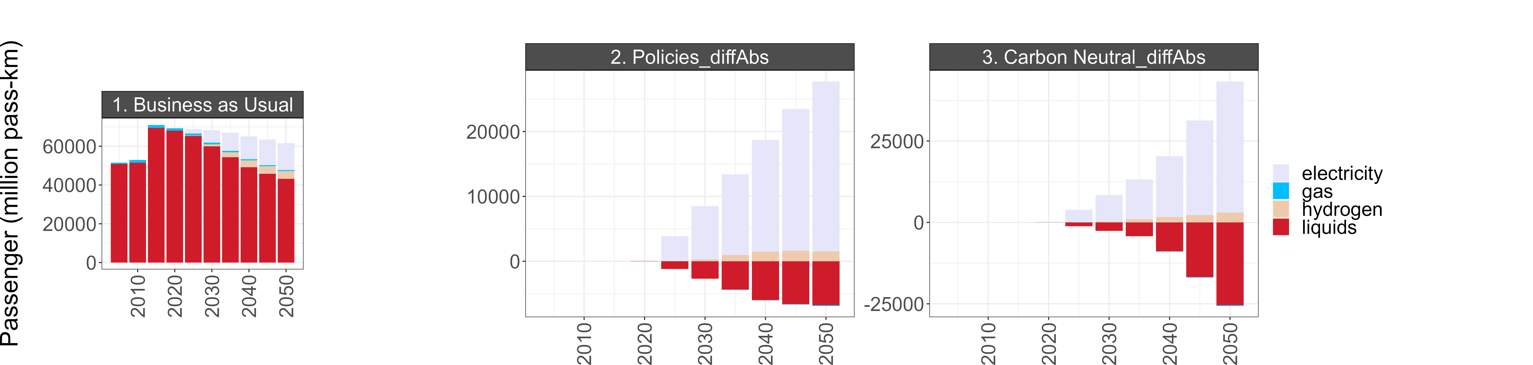
knitr::include_graphics("./markdown_figs/chart_class_pass_fuel.png")

Passenger energy consumption by fuel in Malaysia

knitr::include_graphics("./markdown_figs/chart_class_diff_absolute_pass_fuel.png")

BAU energy consumption (left) and the difference between BAU and the Policies and Carbon Neutral scenarios

7.2.2.3.2 Kuala Lumpur

transport_kl_f <- malaysia %>% 
  filter(param == "transportFreightVMTByFuel",
         region == "KualaLumpur") %>%
  mutate(param = units) %>%
  rchart::chart(save = T, 
                show = F,
                chart_type = c("class_absolute", "class_diff_absolute"),
                scenRef = REF_SCENARIO,
                ncol = 4,
                folder = figure_path,
                append = "_freight_fuel_kl",
                size_text = 24)

transport_kl_f <- malaysia %>% 
  filter(param == "transportPassengerVMTByFuel",
         region == "KualaLumpur") %>%
  mutate(param = units) %>%
  rchart::chart(save = T, 
                show = F,
                chart_type = c("class_absolute", "class_diff_absolute"),
                scenRef = REF_SCENARIO,
                ncol = 4,
                folder = figure_path,
                append = "_pass_fuel_kl",
                size_text = 24)

knitr::include_graphics("./markdown_figs/chart_class_freight_fuel_kl.png")

Freight energy consumption by fuel in Kuala Lumpur

knitr::include_graphics("./markdown_figs/chart_class_diff_absolute_freight_fuel_kl.png")

BAU energy consumption (left) and the difference between BAU and the Policies and Carbon Neutral scenarios

knitr::include_graphics("./markdown_figs/chart_class_pass_fuel_kl.png")

Passenger energy consumption by fuel in Kuala Lumpur

knitr::include_graphics("./markdown_figs/chart_class_diff_absolute_pass_fuel_kl.png")

BAU energy consumption (left) and the difference between BAU and the Policies and Carbon Neutral scenarios

7.2.2.4 Industry Energy by Fuel

7.2.2.4.1 Malaysia

industry_energy_my <- malaysia %>% 
  filter(param == "energyFinalSubsecByFuelIndusEJ",
         region == "All of Malaysia") %>%
  mutate(param = units) %>%
  rchart::chart(save = T, 
                show = F,
                chart_type = c("class_absolute", "class_diff_absolute"),
                scenRef = REF_SCENARIO,
                ncol = 4,
                folder = figure_path,
                append = "_indus_fuel",
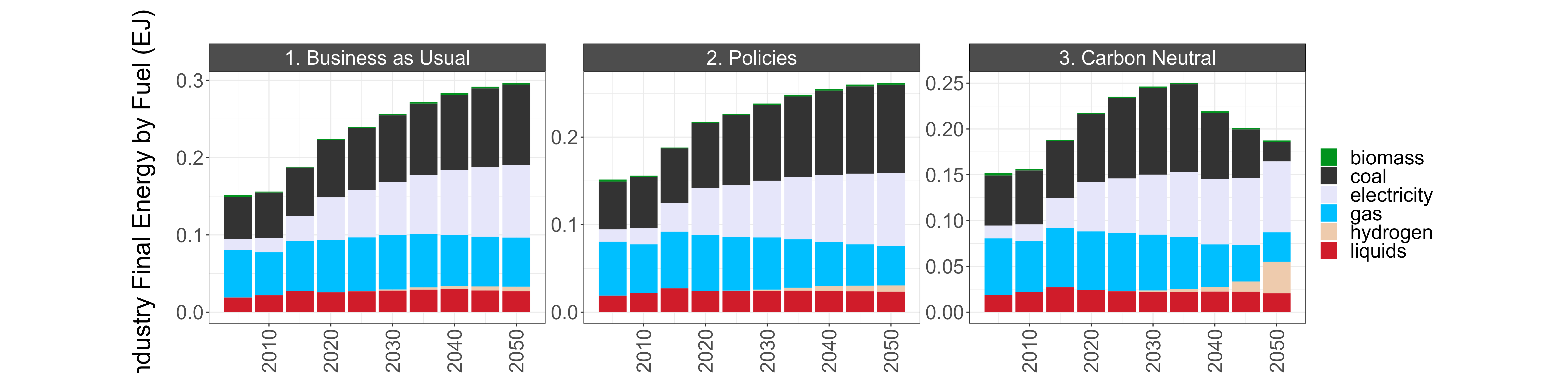
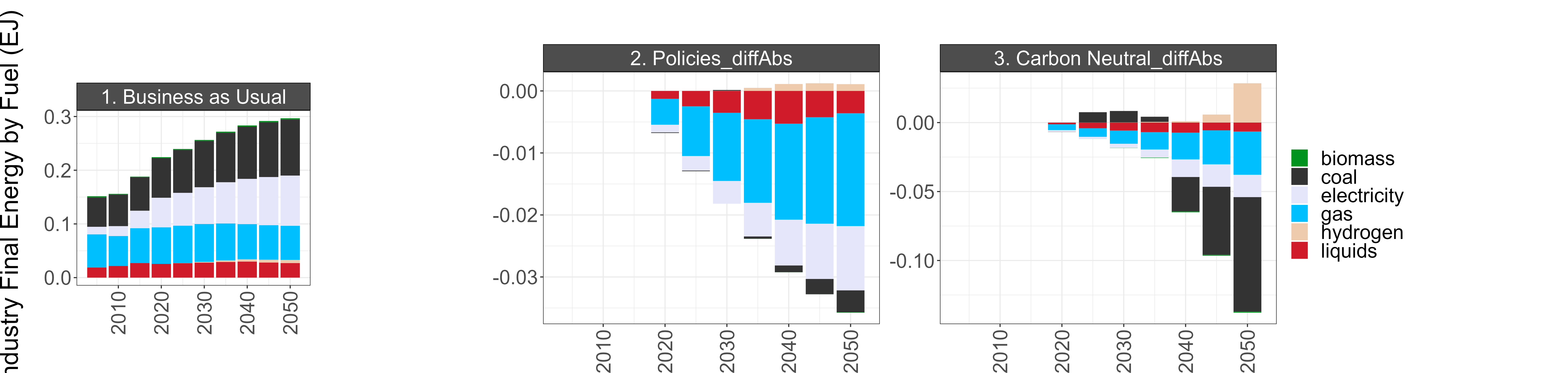
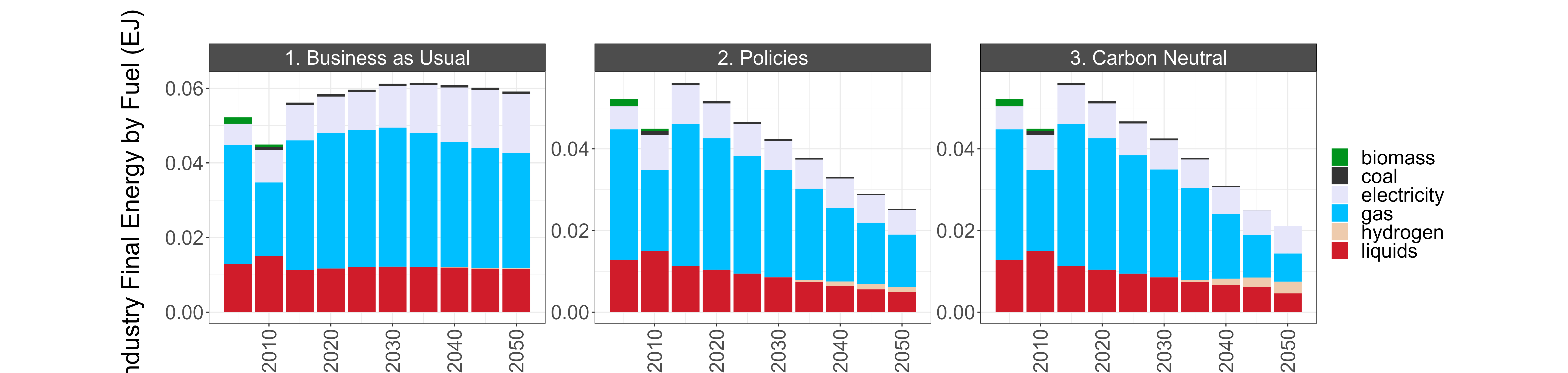
                size_text = 24)

knitr::include_graphics("./markdown_figs/chart_class_indus_fuel.png")

Industry energy consumption by fuel in Malaysia

knitr::include_graphics("./markdown_figs/chart_class_diff_absolute_indus_fuel.png")

BAU energy consumption (left) and the difference between BAU and the Policies and Carbon Neutral scenarios

7.2.2.4.2 Kuala Lumpur

industry_energy_kl <- malaysia %>% 
  filter(param == "energyFinalSubsecByFuelIndusEJ",
         region == "KualaLumpur") %>%
  mutate(param = units) %>%
  rchart::chart(save = T, 
                show = F,
                chart_type = c("class_absolute", "class_diff_absolute"),
                scenRef = REF_SCENARIO,
                ncol = 4,
                folder = figure_path,
                append = "_indus_fuel_kl",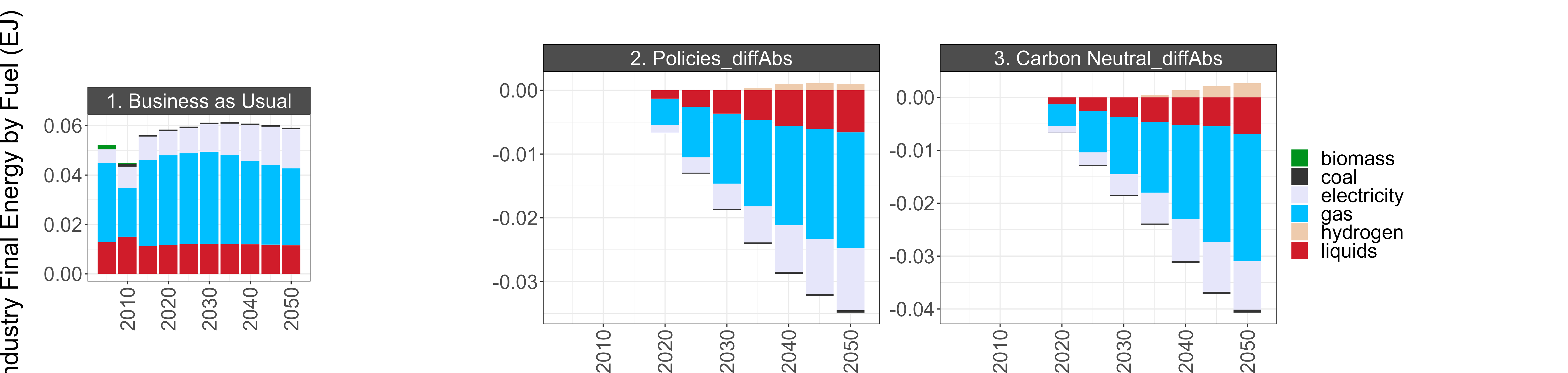
                size_text = 24)

knitr::include_graphics("./markdown_figs/chart_class_indus_fuel_kl.png")

Industry energy consumption by fuel in Kuala Lumpur

knitr::include_graphics("./markdown_figs/chart_class_diff_absolute_indus_fuel_kl.png")

BAU energy consumption (left) and the difference between BAU and the Policies and Carbon Neutral scenarios

8 Assumptions and Validation

8.1 Socioeconomic assumptions

This section details the socioeconomic inputs used to define Malaysia and its subregions, Kuala Lumpur and “Rest of Malaysia,” in GCAM. These metrics include population, GDP, and GDP per capita. Historical and projection data were used when available, otherwise data was calculated using the assumptions described below.

Variable	Assumptions	Data Sources
Population	- Malaysia population used the medium variant projection and historical data from the UN - KL census data gives a value for 2010. All other values were extrapolated and calculated using the growth rates for Malaysia in total - “Rest of Malaysia” values found by subtracting KL numbers from Malaysia	- Malaysia: United Nations - Kuala Lumpur 2010: United Nations
GDP	- Malaysia annual growth rates are applied to KL’s 2020 GDP value to extrapolate historical and future values - “Rest of Malaysia” values found by subtracting KL numbers from Malaysia	- Malaysia, historical: USDA ERS - Malaysia, future: SSP database - Kuala Lumpur 2020: Department of Statistics Malaysia

8.2 Validation of GCAM outputs

This section will compare local Malaysia and KL data (where available) to selected GCAM outputs.

8.2.1 Population and GDP

local_pop <- read.csv("../data/malaysia/local_data_population.csv")
local_gdp <- read.csv("../data/malaysia/local_data_gdp.csv")

local_bau <- bind_rows(local_gdp, local_pop)

gcam_bau <- bind_rows(bau, policies, carbon_neutral) %>%
  filter(param == c("pop", "gdp"),
         region %in% c("Malaysia", "KualaLumpur"),
         scenario == "Ref") %>%
  mutate(param = units,
         scenario = "GCAM Reference",
         year = x)

bau_valid <- bind_rows(local_bau, gcam_bau)

# Plot for Malaysia
bau_valid %>% 
  filter(region == "Malaysia") %>%
  ggplot(aes(x = year, y = value, color = scenario)) + 
  geom_line(size = 1) +
  facet_wrap(~param, scales = "free") +
  ggtitle("Malaysia") +
  scale_color_manual(values = c("darkred", "darkblue")) +
  theme_light()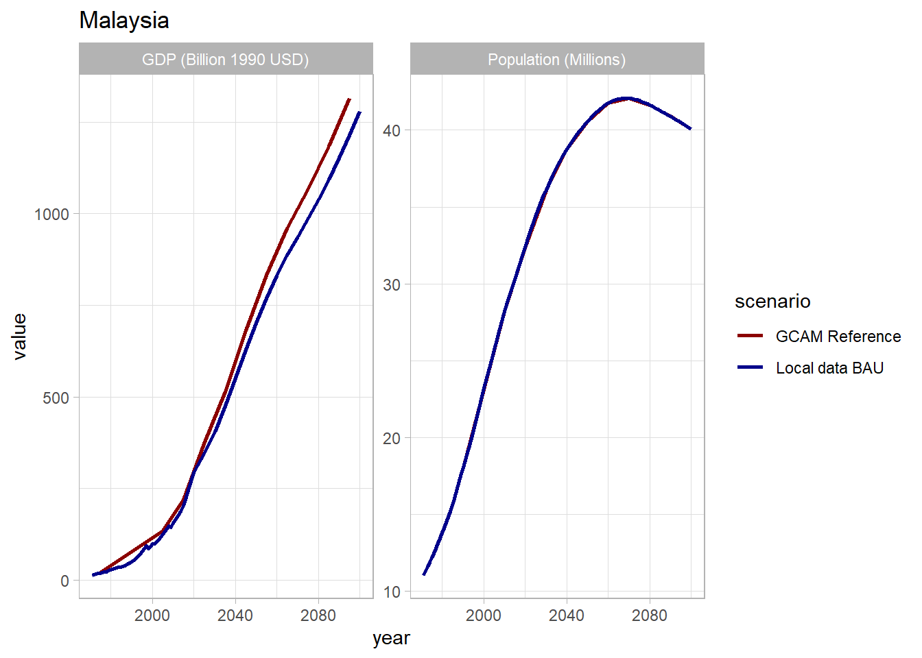

# Plot for KL
bau_valid %>% 
  filter(region == "KualaLumpur") %>%
  ggplot(aes(x = year, y = value, color = scenario)) + 
  geom_line(size = 1) +
  facet_wrap(~param, scales = "free") +
  ggtitle("Kuala Lumpur") +
  scale_color_manual(values = c("darkred", "darkblue")) +
  theme_light()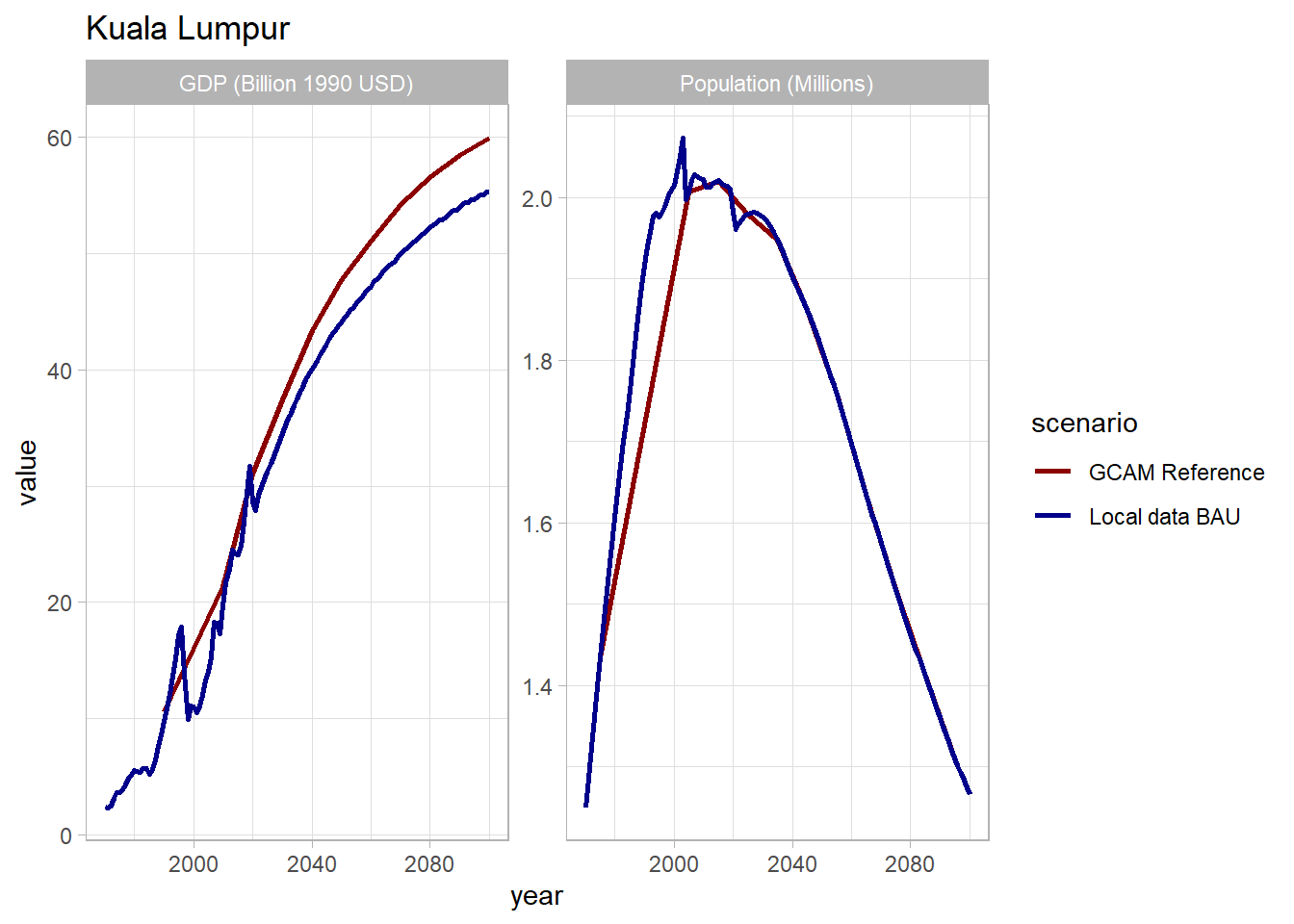

WORK IN PROGRESS - DO NOT CITE