GCAM v8.2 Documentation: GCAM Policies
Documentation for GCAM
The Global Change Analysis Model
View the Project on GitHub JGCRI/gcam-doc
GCAM Policies
One of GCAM’s uses is to explore the implications of different future policies. There are a number of types of policies that can be easily modeled in GCAM. The most common of these are discussed below. Additionally, starting with GCAM v5.2, we have provided a configuration_policy.xml file to help users set up emissions policies. This configuration includes a near-term CO2 price (spa14_tax.xml), a long-term CO2 price (carbon_tax_0.xml), and a file to link both to CO2 emissions in GCAM (2025_target_finder.xml).
Table Of Contents
- Emissions-Related Policies
- Land-Use Policies
- Energy Production Policies
- Emissions-Related Policies
- Calculating Emissions Policy Costs
Emissions-Related Policies
There are three main policy approaches that can be applied in GCAM to reduce emissions of CO2 or other greenhouse gases: carbon or GHG prices, emissions constraints, or climate constraints. In all cases, GCAM implements the policy approach by placing a price on emissions. This price then filters down through all the systems in GCAM and alters production and demand. For example, a price on carbon would put a cost on emitting fossil fuels. This cost would then influence the cost of producing electricity from fossil-fired power plants that emit CO2, which would then influence their relative cost compared to other electricity generating technologies and increase the price of electricity. The increased price of electricity would then make its way to consumers that use electricity, decreasing its competitiveness relative to other fuels and leading to a decrease in electricity demand. The three policy approaches are described below.
-
Carbon or GHG prices: GCAM users can directly specify the price of carbon or GHGs. Given a carbon price, the resulting emissions will vary depending on other scenario drivers, such as population, GDP, resources, and technology. See example.
-
Emissions constraints. GCAM users can specify the total amount of emissions (CO2 or GHG) as well. GCAM will then calculate the price of carbon needed to reach the constraint in each period of the constraint.
-
Climate constraints: GCAM users can specify a climate variable (e.g., concentration or radiative forcing) target for a particular year. Users determine whether that target can be exceeded prior to the target year. GCAM will adjust carbon prices in order to find the least cost path to reaching the target. (Note that this type of policy increases model run time significantly.)
Linked Emission Markets
Emissions prices of different GHGs can be linked together for a multi-gas policy using the linked-ghg-policy object. For example, in the default linked_ghg_policy.xml file in the GCAM release, all non-CO2 GHGs are linked to the market for CO2. Also, see example
The parameter price-adjust is used to convert prices (e.g., 100 year GWPs in the default set-up) and demand-adjust is used to convert demand units (e.g., to common units of carbon equivalents). These can be changed by year if desired.
Setting price-adjust to zero means that there is no economic feedback for the price of this GHG. MAC curves, however, will still operate under the default set-up (whereby MAC curves are driven by CO2 prices). This can be changed separately for energy/industrial/urban CH4, agricultural CH4 (CH4_AGR), and CH4 from agricultural waste burning (CH4_AWB), LUC CO2 emissions (e.g. CO2_LUC).
Note that you must first create a policy by reading in a
This flexibility allows CO2-only, CO2-equivalent, or non-CO2 markets/constraints for various “baskets” of emissions as needed.
Note that the GCAM default set-up includes economic feedbacks for methane and nitrous oxide. This is an idealized assumption, but might not happen in real-world policies. For example, in many current systems agricultural emissions are offsets only – e.g., they get paid to reduce emissions, but are not charged for any remaining emissions. (So to simulate this type of policy, price-adjust would be set to zero).
Markets For non-CO2 Emission Species
Markets in GCAM can be set for any emission species. (e.g., CH4 -only market, NOx market, etc.)
Note that it generally does not make sense to set up an emissions market unless the model has a direct way to reduce emissions. (e.g. you’ve added relevant MAC curves.) For example, in Shi et al. (2017) US electricity sector SO2 and NOx markets were used to represent current policies that cap emissions in certain states. MAC curves for existing power plants were added to allow emissions to change in response to market prices.
xml inputs within the MAC curve that will be needed to set-up new markets are:
| XML Tag | Description |
|---|---|
| market-name | Name of market from which the price used by the MAC curve will be obtained (default = “CO2”) |
| mac-price-conversion | Value to multiply market price by to convert to unit expected by the MAC curve (for example, converting from $/tC to $/tCO2eq) (default = 1) |
| Note | mac-price-conversion can also be set to -1, which is a flag to turn off all use of the MAC curve. This is useful for sensitivity studies. |
| zero-cost-phase-in-time | Number of years over which to phase-in “below-zero” MAC curve reductions (default = 25 years) |
Energy Production Policies
There are times in which users would like to explore the implications of a constraint on production or a minimum production requirement. This capability allows GCAM users to model policies such as renewable portfolio standards and biofuels standards. Across sectors, these constraints must be applied as quantity constraints, but they can be applied as share constraints within individual sectors (e.g., fraction of electricity that comes from solar power). In implementing these policies, this can either be a lower bound or upper bound. The model will solve for the tax (upper bound) or subsidy (lower bound) required to reach the given constraint. Examples of bioenergy constraints are provided.
Land-Use Policies
There are a number of ways that policies can be applied directly to influence the land sector in GCAM. These include the following.
-
Protected Lands: With this policy, GCAM users can set aside a fraction of natural land, removing it from economic competition. This land cannot be converted to crops, pasture, or any other land type. This is similar to real-world policies such as reducing emissions from deforestation and forest degradation (REDD). The default in GCAM is to protect 90% of all non-commercial ecosystems.
-
Valuing carbon in land: When applying a price on carbon through any of the emissions-related policy approaches, GCAM users can choose whether that price extends to land use change CO2 emissions. This policy is modeled as a subsidy to land-owners for the holding carbon stocks as opposed to a price on the emissions themselves.
- Bioenergy constraints: GCAM users can impose constraints on bioenergy within GCAM. Under such a policy, GCAM will calculate the tax or subsidy required to ensure that the constraint is met. By default two bioenergy related constraints are enabled in GCAM and described below. Alternative approaches could be used for more direct constraints as show in the examples.
- Negative emissions budget: This constraint limits the total gross value of all negative emissions, be it bioenergy or otherwise, to a certain fraction of GDP as defined by
energy.NEG_EMISS_GDP_BUDGET_PCTin constants.R. To enforce the constraint the model will scale back the value of the subsidy given to bioenergy to stay within the budget. Thus limiting the value but not necessarily the quantity of negative emissions. Note this budget is also applied to the valuation of carbon in land when running such a policy, however the actual value of those emissions are not included in this budget at the moment. - Biomass externality cost: We include an additional constraint which is meant to represent the costs paid for various externalities resulting from large scale production of purpose grown bioenergy crops. This constraint is represented with an increasing cost with higher levels of production as defined in A27.GrdRenewRsrcCurves.csv.
- Negative emissions budget: This constraint limits the total gross value of all negative emissions, be it bioenergy or otherwise, to a certain fraction of GDP as defined by
- Land constraints: GCAM users can constraint the amount of land of a particular type in a given region. Under such a policy, GCAM will calculate the tax or subsidy required to ensure that the constraint is met. See example.
Calculating Emissions Policy Costs
The cost of GHG emissions mitigation is a concept that is not uniquely defined. A wide range of measures are used in the literature. These include, the price of carbon (or as appropriate given the policy) needed to achieve a desired emission mitigation goal, reduction in Gross Domestic Product (GDP), consumption loss, deadweight loss, and equivalent variation. Beyond that the concept of net cost, which includes the benefits of emissions mitigation as well as the resource cost of emissions reduction and the social cost of carbon are also encountered. GCAM makes no attempt to calculate the benefits.
In addition to identifying policy prices as one measure of cost, GCAM employs the “deadweight loss” approach to measuring welfare loss from emissions mitigation efforts. GCAM employs the deadweight loss approach for several reasons. First, the deadweight loss approach is numerically straight forward to calculate in GCAM. Second, the deadweight loss approach provides a computationally tractable method to measuring the change in welfare, though it is only an approximation. In principle the equivalent variation is the right approach to measure an individual’s loss in welfare. Equivalent variation measures the minimum amount of income that would be needed to leave consumers just as happy with the new price (e.g. carbon tax) as without. However, its calculation requires either knowledge of all of society’s individual preference functions or the existence of a well-ordered set of social preferences, a requirement that Arrow (1950) demonstrated to be impossible under ordinary circumstances. Third, the deadweight loss approach takes advantage of GCAM’s detailed technological characterization.
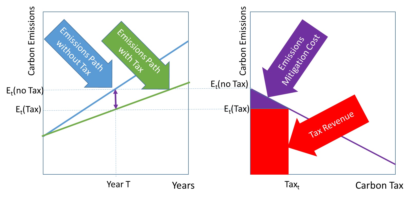
A detailed description of the method used in GCAM is documented in Bradley et al. (1991). In general, the approach is as follows. GCAM calculates the cost of emissions mitigation at each GCAM time step. For example in the figure below, the cost of moving from a reference path without a carbon tax (blue) to the emissions path with a carbon tax (green) in period T can be calculated simply. Successive scenarios with fixed carbon taxes in period T are run. The associated emissions are recorded for each carbon tax. The cost is calculated as the area of the purple triangle, which is the integral of each emissions mitigation step weighted by the carbon tax that was required to deliver the reduction. The final ton of carbon emissions is the most expensive ton, because it is assumed that for a carbon tax, emissions mitigation occurs with the least expensive tons being reduced first. The final ton of carbon is simply the carbon tax rate itself. The tax revenue can be calculated as the tax rate times the remaining emissions, shown in red below.
As discussed in Bradley et al. (1991) and demonstrated in Calvin et al. (2014), the approach can be used to calculate costs for a wide range of heterogeneous non-price policies. While conceptually similar to the simple approach above, the other is tedious. Similarly, the deadweight loss approach can be used to calculate the cost of policies other than carbon taxes. It is completely general Mankiw & Hakes (2012).
The approach is employed at each GCAM time step. Costs occurring between time steps is inferred by interpolation. Costs over time can be summed. Costs can be summed with or without discounting. But, the GCAM user needs to be aware of the implications of whatever approach is employed.
The deadweight loss approach is not without its limitations. While the numerical calculation is simple for a uniform carbon tax (or a cap-and-trade regime), more complex policies are more tedious to represent. Second, there is no link back to the macro-economy. Changes of the magnitude associated with stringent climate policies will have macro-economic consequences. Those consequence will, in turn affect the scale of economic activity. Third, there is no way to calculate the effects of alternative uses of tax revenue or carbon permit allocations.
Note that calculation of policy costs is currently only supported for polices pegged to CO2 prices.
References
[Arrow 1950] Arrow, Kenneth J. (1950). “A Difficulty in the Concept of Social Welfare” (PDF). Journal of Political Economy. 58 (4): 328–346. doi:10.1086/256963. Link
[Bhattacharya 2001] Bhattacharya, Jay. (2001). Three measures of the change in welfare. Link
[Bradley et al. 1991] Bradley, Richard A., Edward C. Watts, and Edward R. Williams. Limiting net greenhouse gas emissions in the United States. No. DOE/PE-0101-Vol. 2. USDOE Office of Policy, Planning and Analysis, Washington, DC (United States). Office of Environmental Analysis, 1991. Link
[Calvin et al. 2014] Calvin, Katherine, Jae Edmonds, Bjorn Bakken, Marshall Wise, Son H. Kim, Patrick Luckow, Pralit Patel, Ingeborg Graabak. (2014). The EU20-20-20 energy policy as a model for global climate mitigation. Climate Policy. Link
[Mankiw & Hakes 2012] Mankiw, N. and David Hakes (2012). Principles of microeconomics. South-Western Cengage Learning.
[Shi et al. 2017] Shi W, Ou Y, Smith S J, Ledna C M, Nolte C G, Loughlin D H 2017. “Projecting state-level air pollutant emissions using an integrated assessment model: GCAM-USA” Applied Energy 208 511–521. doi: 10.1016/j.apenergy.2017.09.122. Link