Install

- Download and install:
- R (https://www.r-project.org/)
- R studio (https://www.rstudio.com/) (Optional)
- In R or R studio:
install.packages("devtools")
devtools::install_github("JGCRI/rmap")
Additional steps for UBUNTU from a terminal
sudo add-apt-repository ppa:ubuntugis/ppa
sudo apt-get update
sudo apt-get install -y libcurl4-openssl-dev libssl-dev libxml2-dev libudunits2-dev libgdal-dev libgeos-dev libproj-dev libavfilter-dev  libmagick++-dev
Additional steps for MACOSX from a terminal
brew install pkg-config
brew install gdal
brew install geos
brew install imagemagick@6
Input Structure
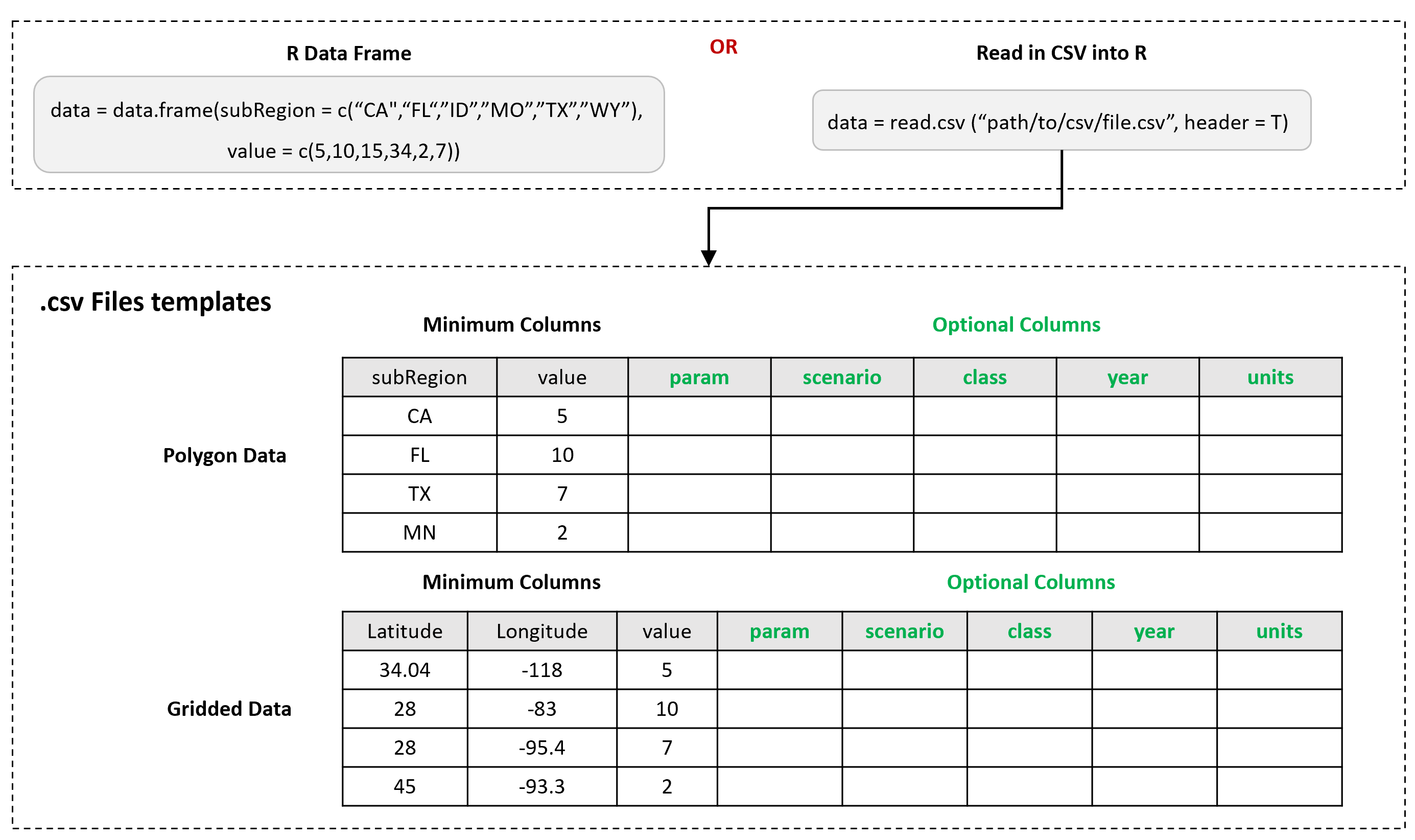
The main input is the data argument in the
map() function. This will be an R table which can be
created within R or read in from a csv file as shown below. As shown
later if a shape file (SpatialPolygonDataFrame) is provided
as the data argument (see Section Built-in Maps)
then the map() function will produce a map without any
value data.
Custom Columns
Users can also assign other column names to x (the time
dimension), class, subRegion,
scenario and value if desired using the
x, class, subRegion,
scenario and value arguments as follows:
library(rmap);
data = data.frame(my_column_1 = c("CA","FL","ID","CA","FL","ID","CA","FL","ID","CA","FL","ID"),
                  my_column_2 = c(5,10,15,34,22,77,15,110,115,134,122,177),
                  my_column_3 = c(2010,2010,2010,2020,2020,2020,2010,2010,2010,2020,2020,2020),
                  my_column_4 = c("class1","class1","class1","class1","class1","class1",
                                  "class2","class2","class2","class2","class2","class2"),
                  my_column_5 = c("my_scenario","my_scenario","my_scenario","my_scenario","my_scenario","my_scenario",
                                  "my_scenario","my_scenario","my_scenario","my_scenario","my_scenario","my_scenario"))
rmap::map(data,
          subRegion = "my_column_1",
          value = "my_column_2",
          x = "my_column_3",
          class = "my_column_4",
          scenario = "my_column_5")
Cleaning Data
Users will need to check that the names of the regions in their data
tables match those of the subRegion column of the built-in maps or a custom shapefile
if they are using one. Sometimes user data may have a few names that
have different spelling or accents and these will be flagged when rmap
plots the maps. Users can then go back to their original data and fix
those regions as shown in the example below.
library(rmap); library(dplyr)

# Create data table with a misspelled subRegion
data = data.frame(subRegion = c("Italy","Spain","Greice"),
                  value = c(10,15,34))

# Plot data
rmap::map(data,labels = T, title = "Misspelled subRegion 'Greice'")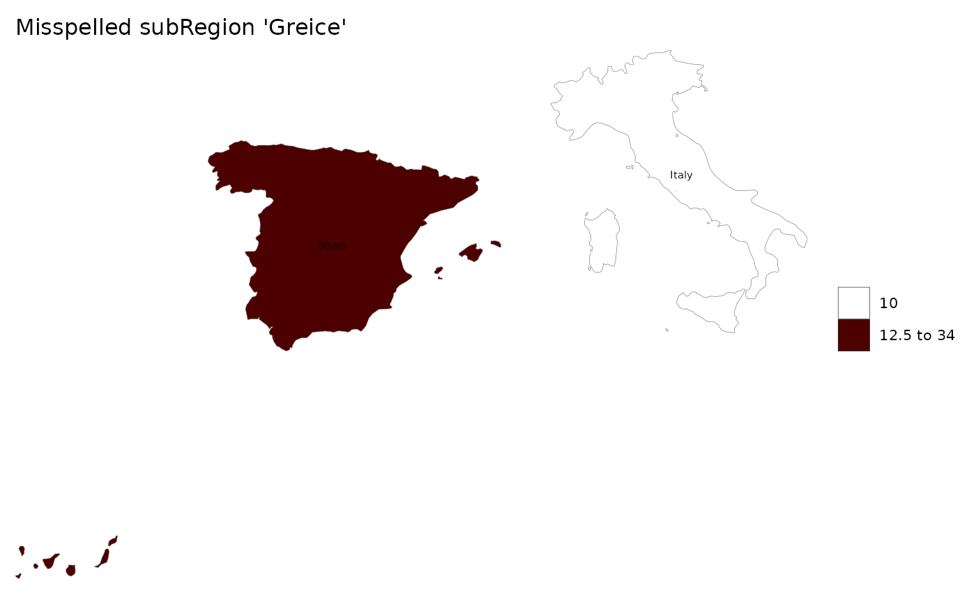
# Will return: 'Warning: subRegions in data not present in shapefile are: Greice'
# As well as the built-in map used: 'Using map: mapCountries'

# Check the subRegions in the map used
rmap::mapCountries$subRegion%>%unique()%>%sort()

# Fix the subRegion that was misspelled
data = data.frame(subRegion = c("Italy","Spain","Greece"),
                  value = c(10,15,34))

# Re-plot cleaned data
rmap::map(data,labels = T, title = "Correctly spelled subRegion 'Greece'")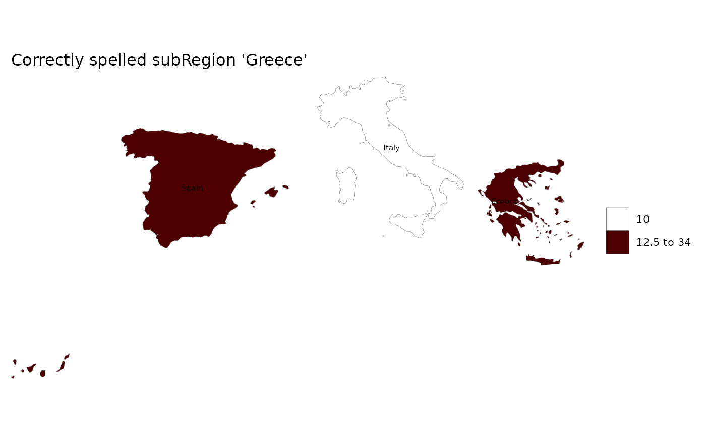
Output Formats
The output of the map() function is a named list with
all maps and animations created in the function. The elements of the
list can be called individually and re-used as layers in new maps as
decribed in the Layers section. Since the output
maps are ggplot elements all the features of the map can
easily be modified using the taditional ggplot2 theme
options. Examples are provided in the Themes
section.
library(rmap);
my_map_list <- rmap::map(mapUS49) # my_map_list will contain a list of the maps produced. In this case a single map.
my_map <- my_map_list[[1]] # my_map will be the first map in the list of maps produced
my_map_names <- names(my_map_list) # Will give you a list of the maps produced.
rmap::map(mapUS49) # Will print out the maps to the console as well save the maps as well as the related data tables to a default directory.
rmap::map(mapUS49, show = F) # will return a map and save to disk without printing to console.
rmap::map(mapUS49, folder = "myOutputs") # Will save outputs to a directory called myOutputs
rmap::map(mapUS49, save = F) # Will simply print the maps to the console and not save the maps to file.
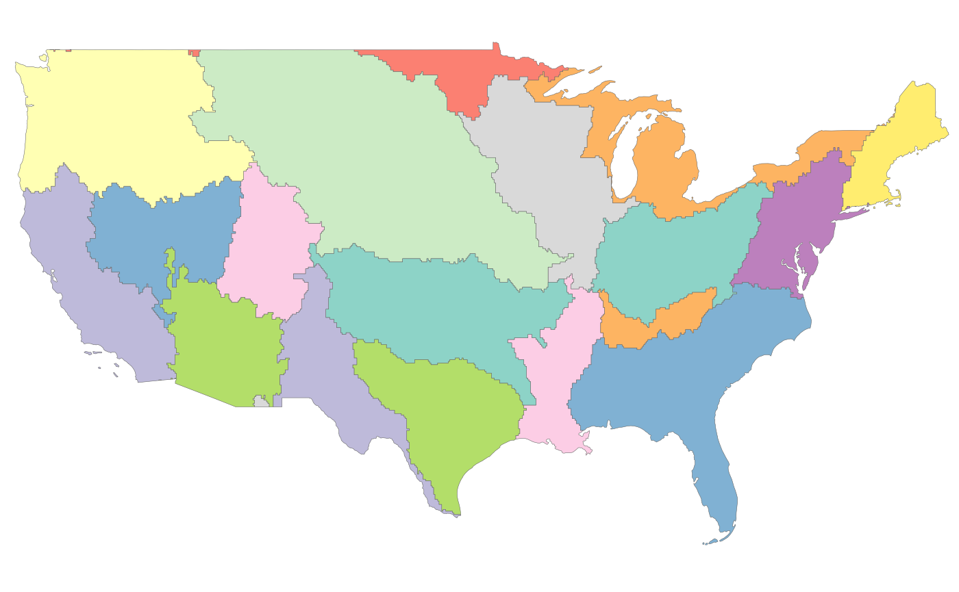
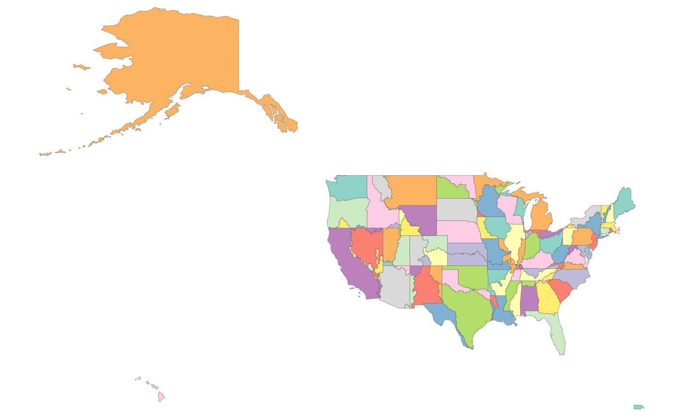
Built-in Maps
rmap comes with a set of preloaded maps. A full list of maps is
available in the reference list of maps. The
pre-loaded maps are all sf objects. Each map comes with a
data column named subRegion. For each map the data
contained in the shape and the map itself can be viewed as follows:
library(rmap);
head(mapUS49) # To view data for chosen map
plot(mapUS49[,"subRegion"]) # plot regular sf object
# Plot Using rmap
rmap::map(mapUS49)
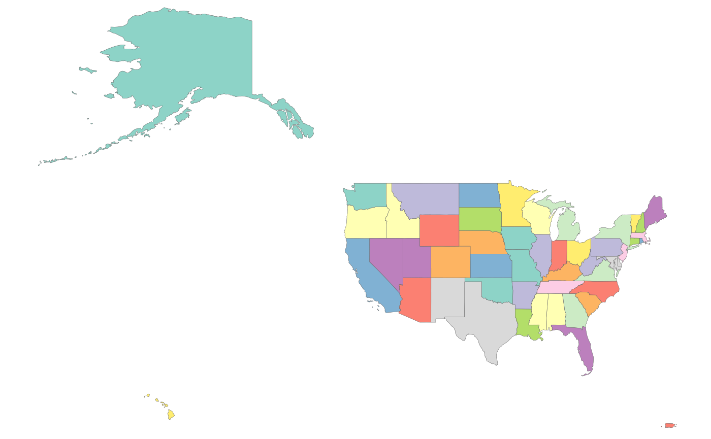
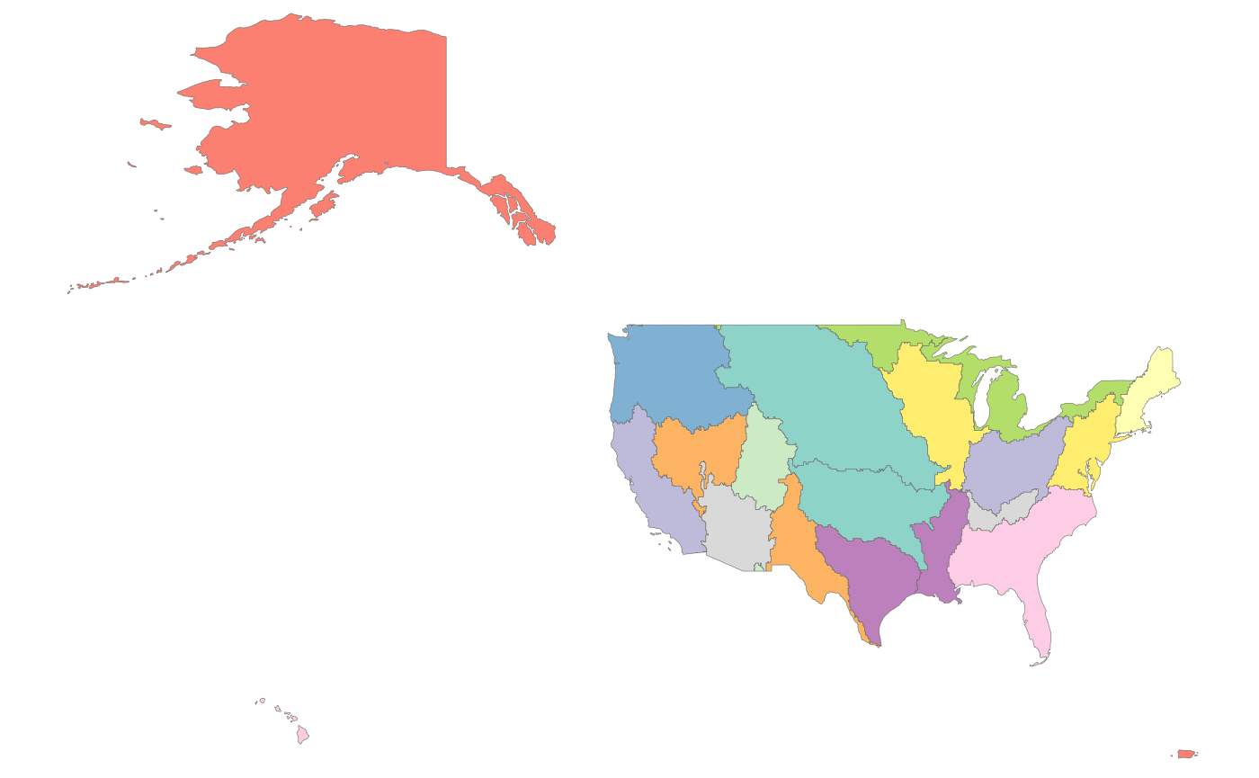
rmap::map(mapUS52)
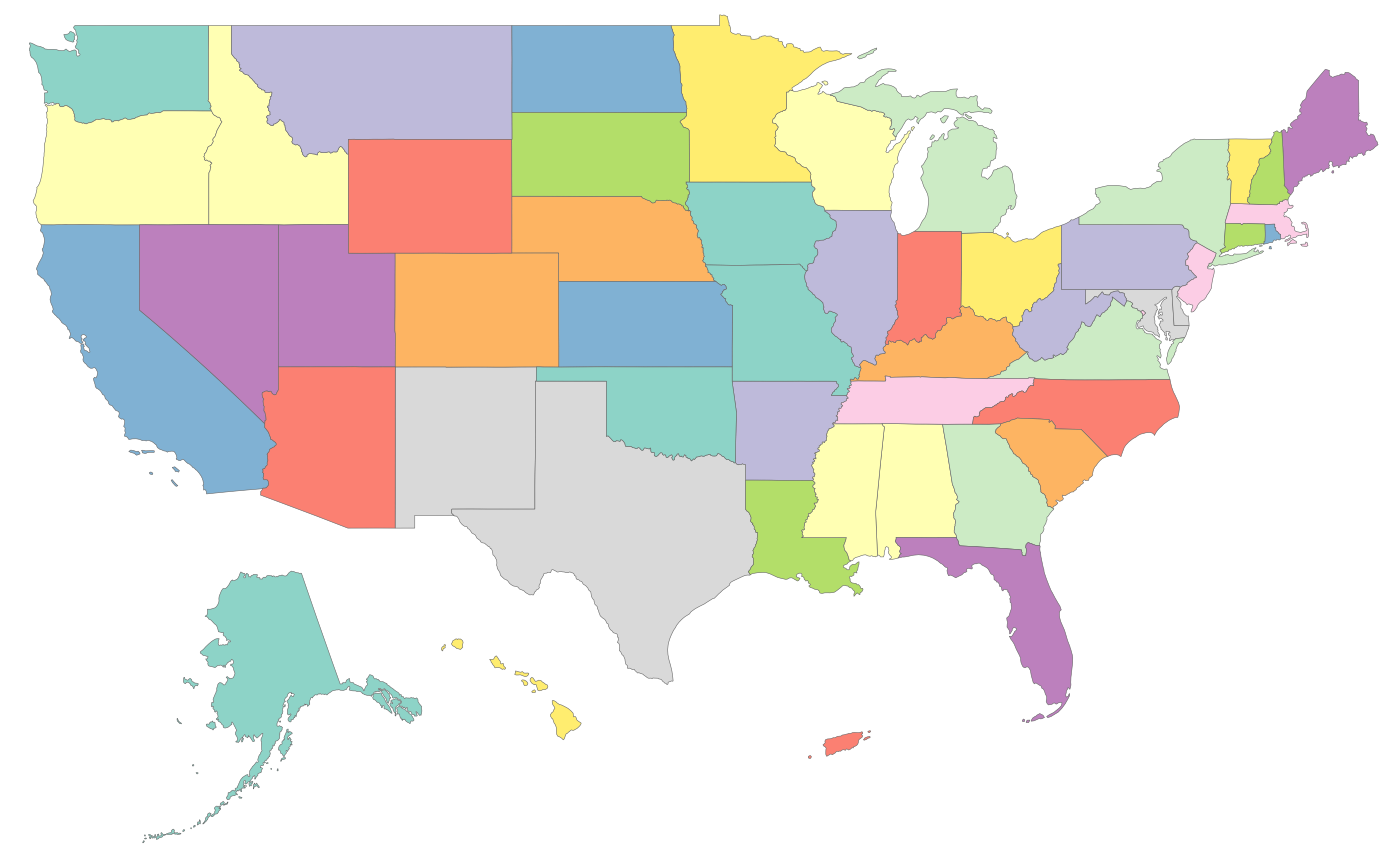
rmap::map(mapUS52Compact)
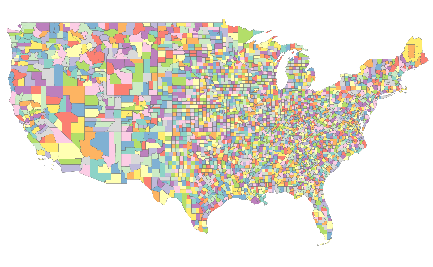
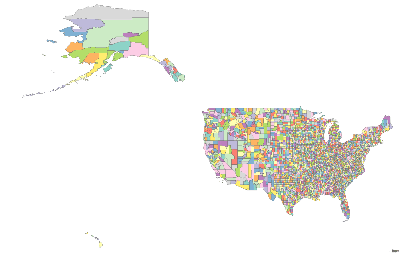
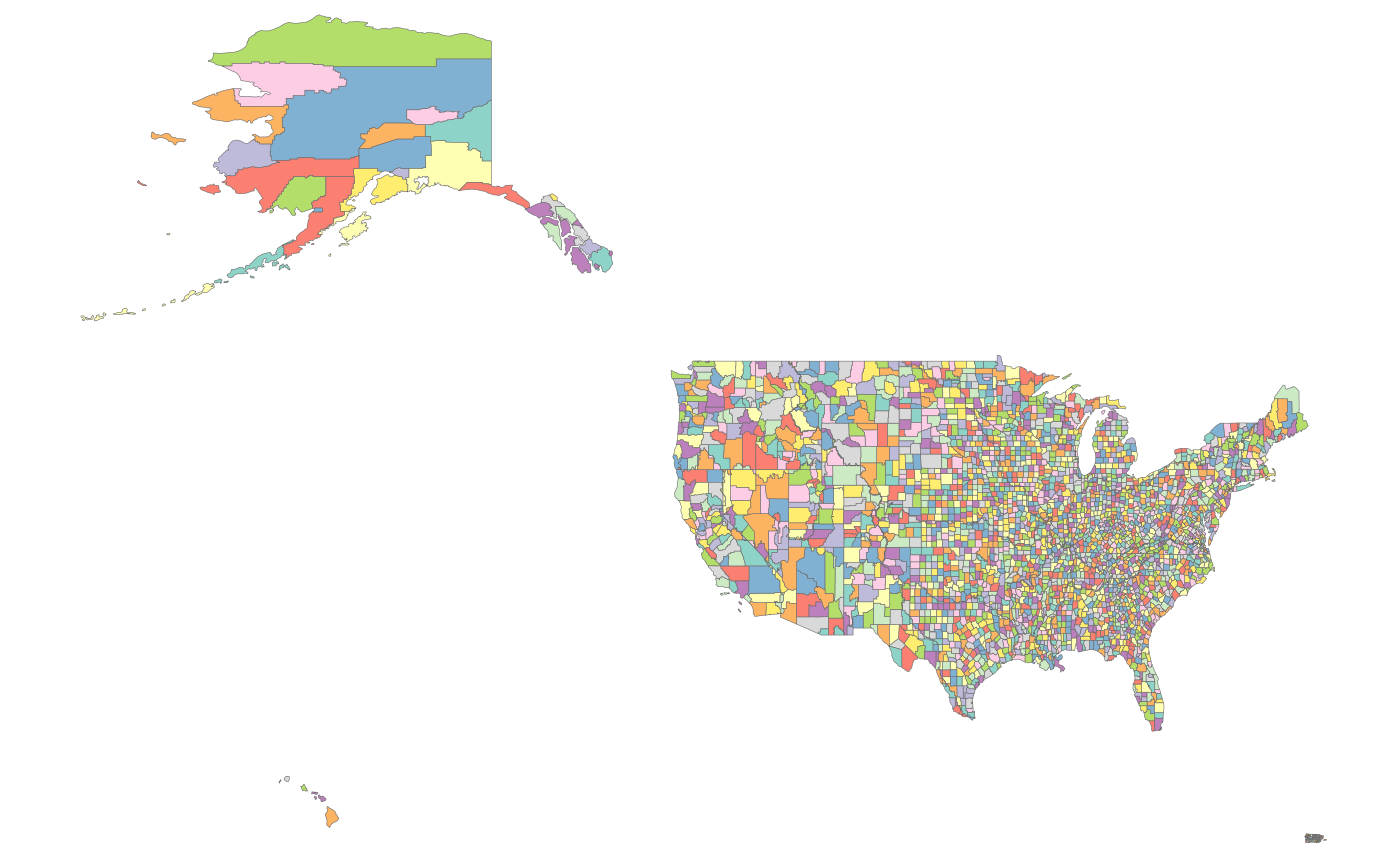
rmap::map(mapUS49County)
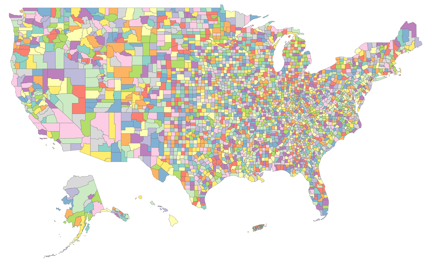
rmap::map(mapUS52County)
rmap::map(mapUS52CountyCompact)
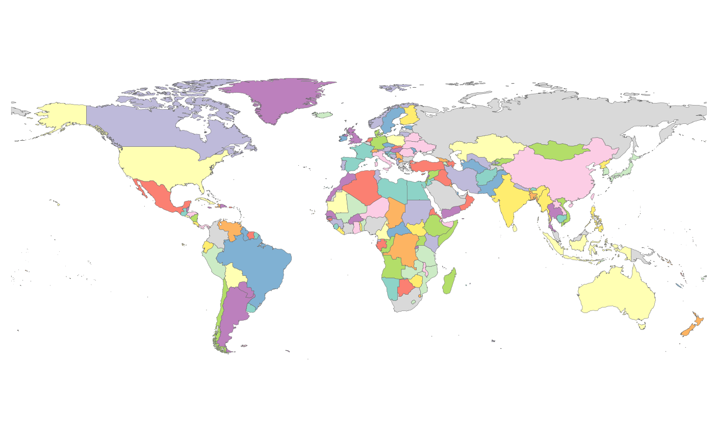
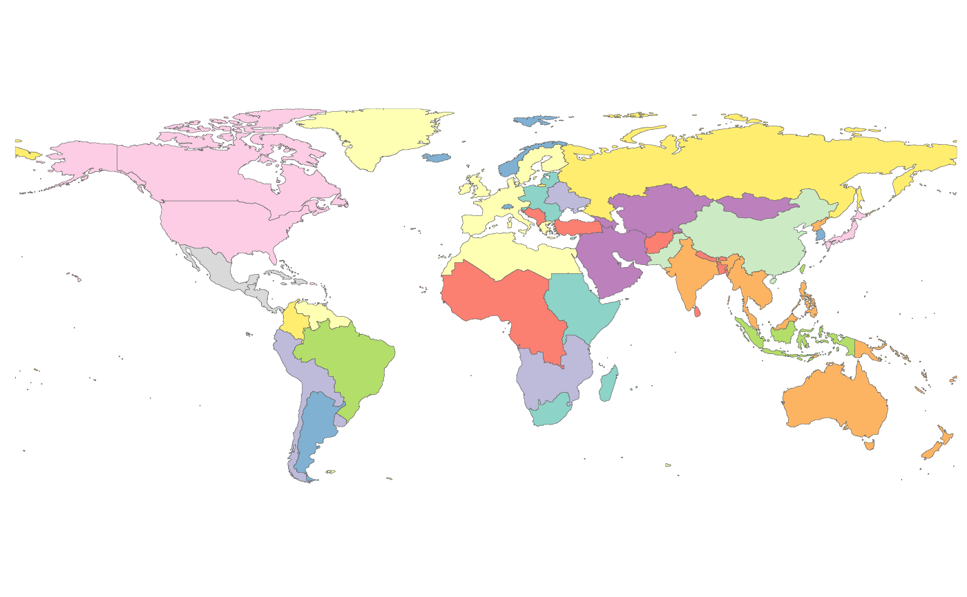
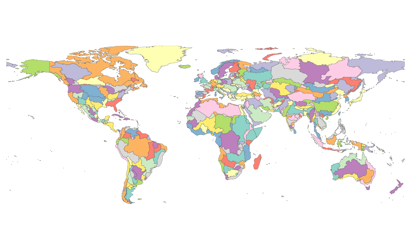
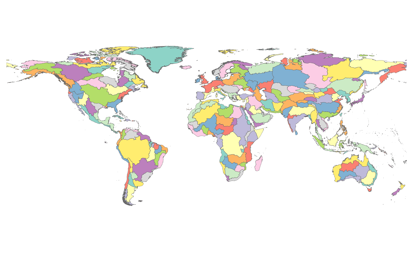
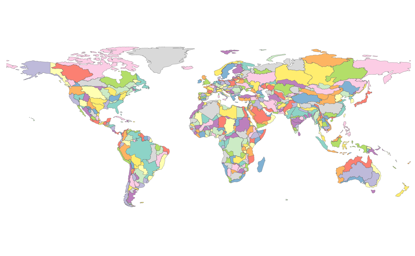
rmap::map(mapCountries)
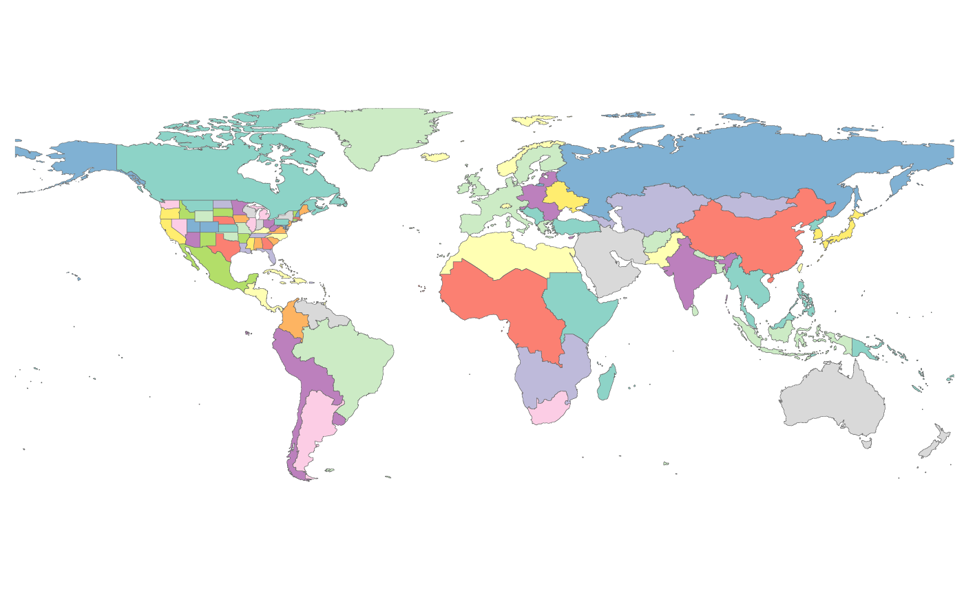
rmap::map(mapCountriesUS52)
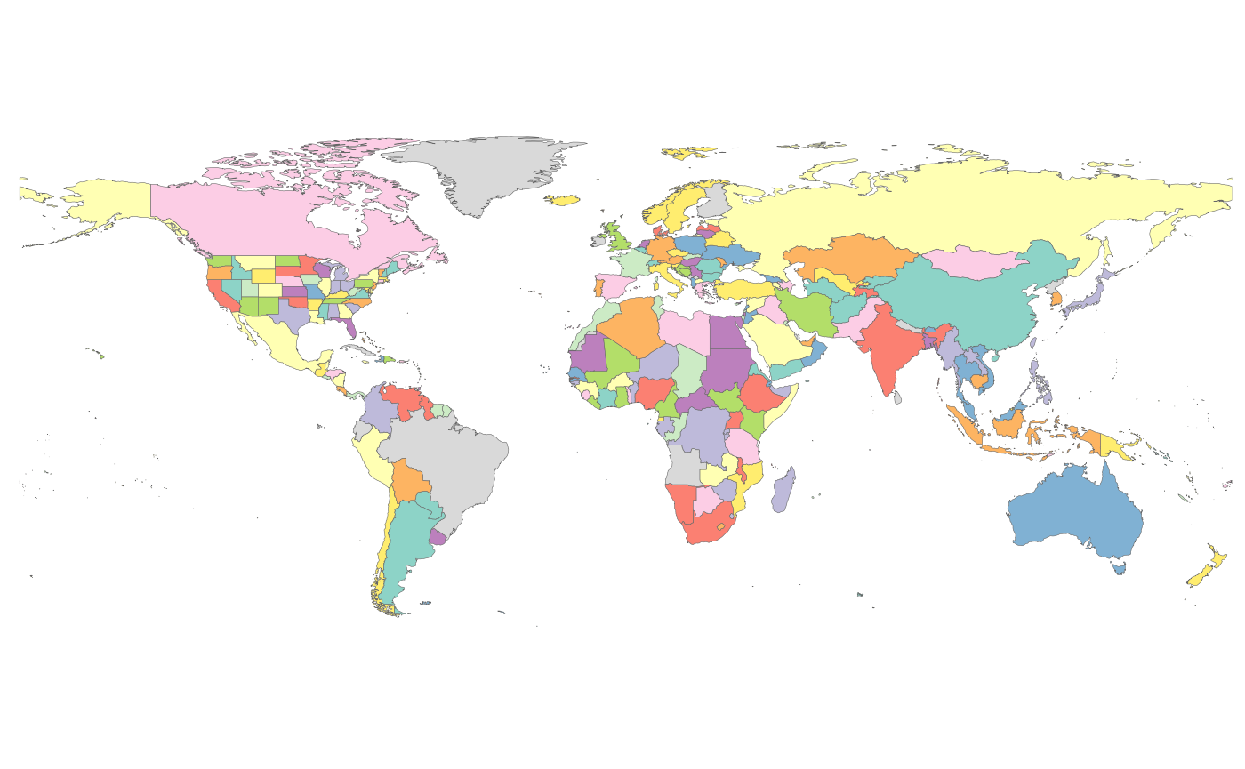
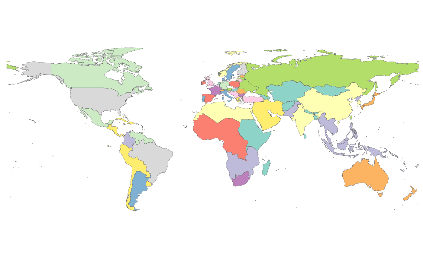
rmap::map(mapGCAMReg32)
rmap::map(mapGCAMReg32US52)
rmap::map(mapGCAMBasins)
rmap::map(mapGCAMBasinsUS49)
rmap::map(mapGCAMBasinsUS52)
rmap::map(mapGCAMLand) # Intersection of GCAM 32 regions and GCAM Basins
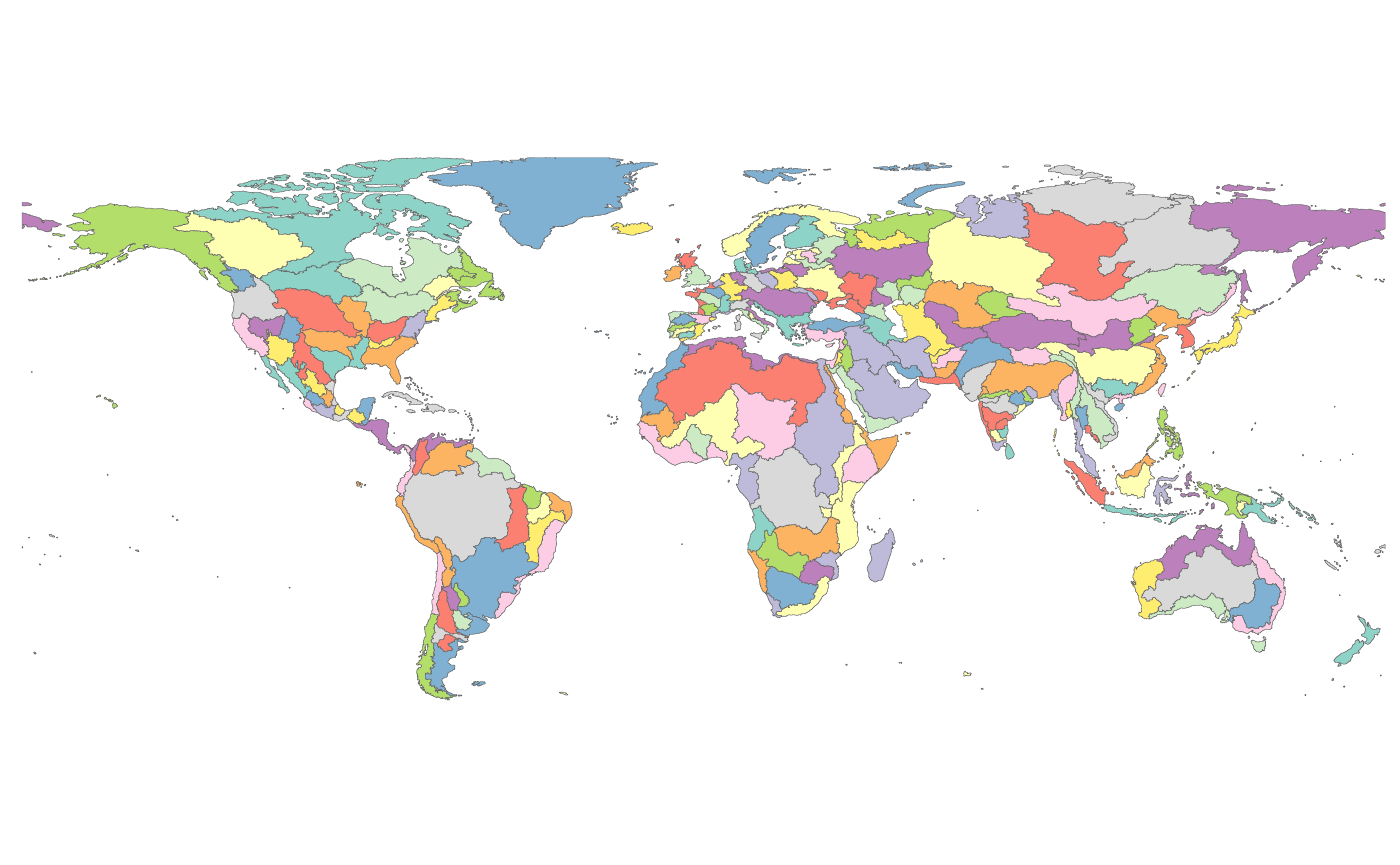
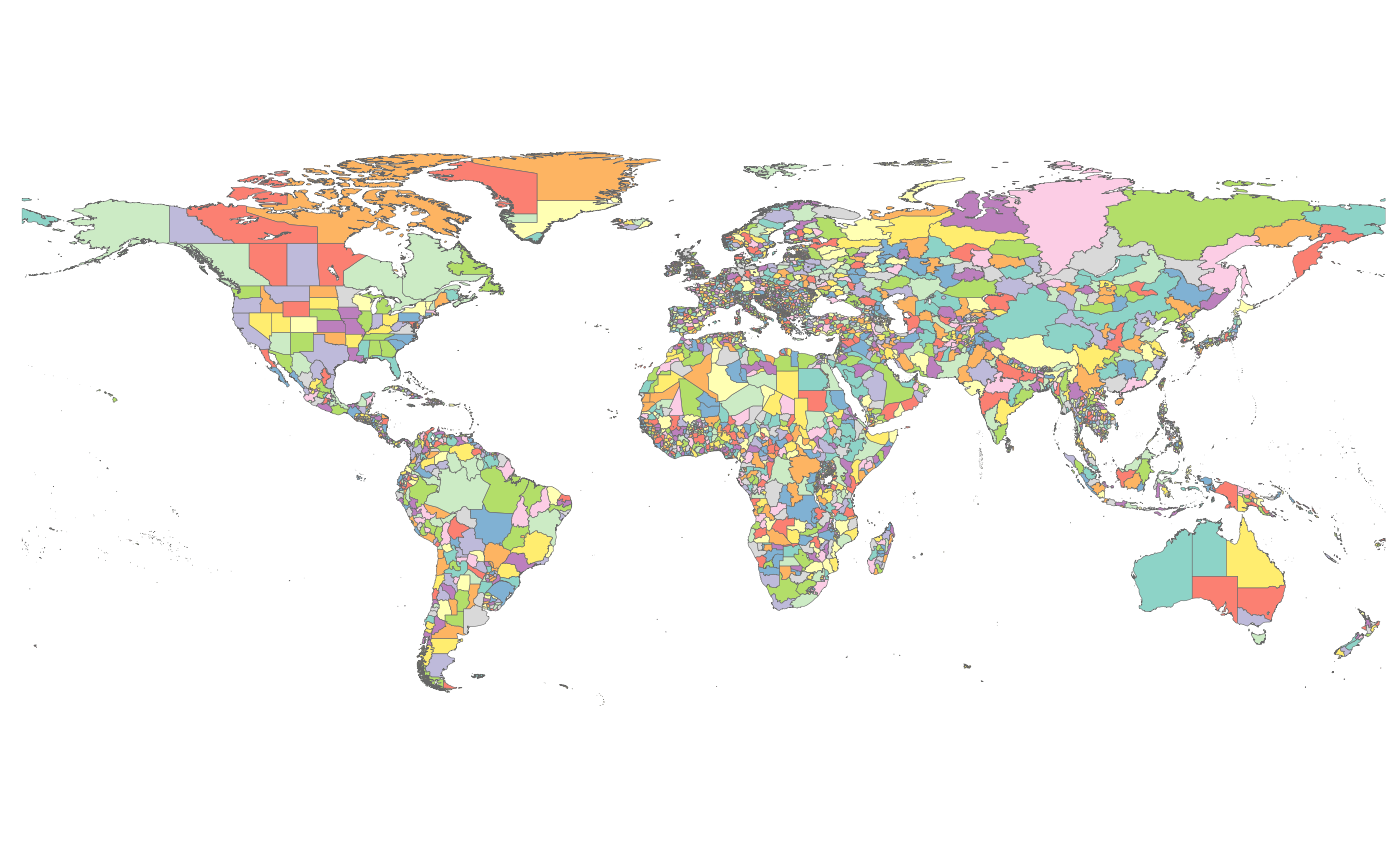
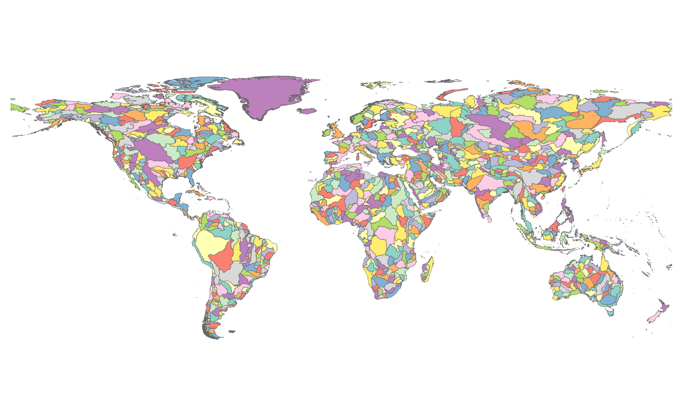
rmap::map(mapStates)
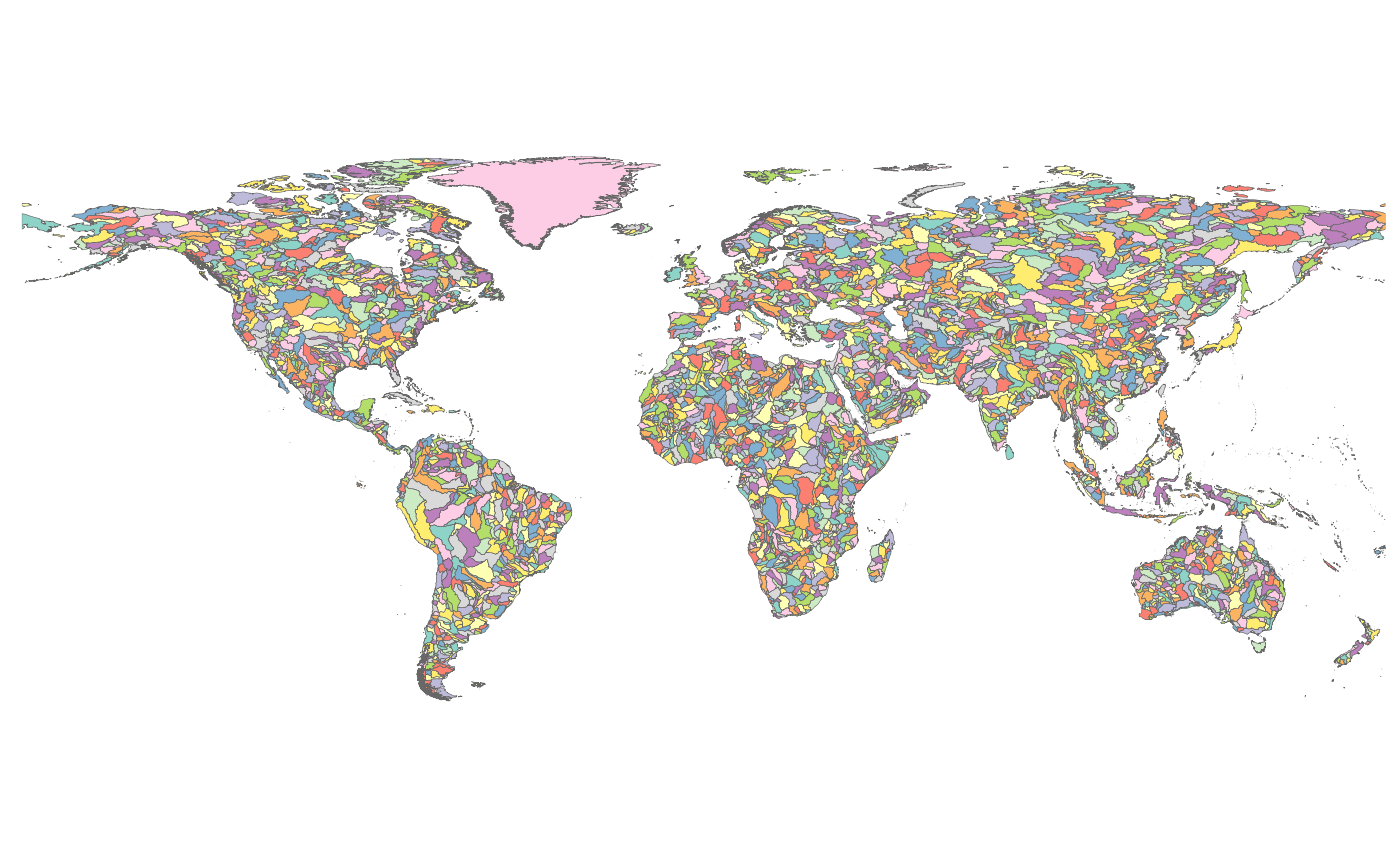
rmap::map(mapHydroShed1)
rmap::map(mapHydroShed2)
rmap::map(mapHydroShed3)
rmap::map(mapIntersectGCAMBasinCountry)
rmap::map(mapIntersectGCAMBasinUS52)
rmap::map(mapIntersectGCAMBasinUS52County)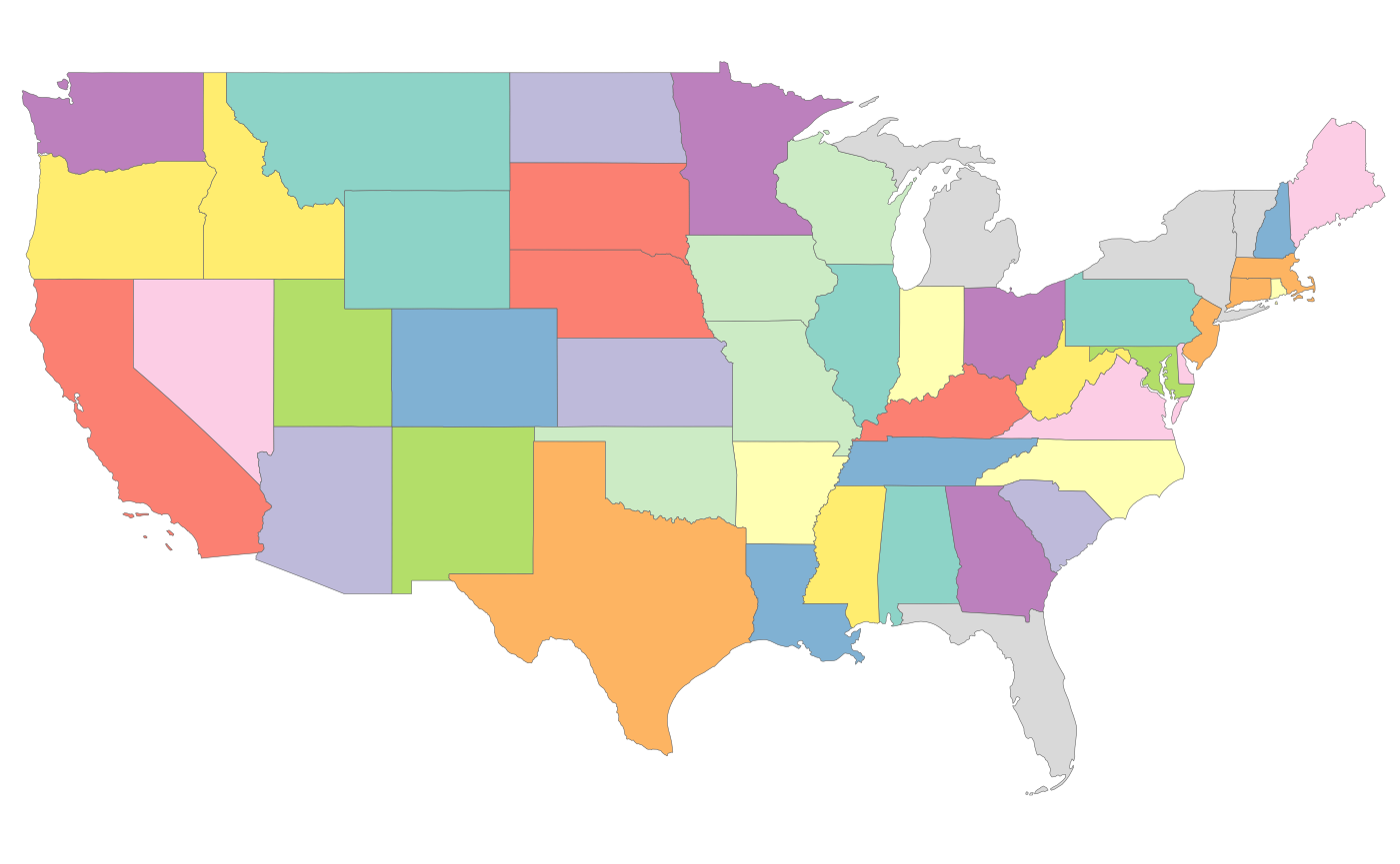
Projections
Users can change the projection of maps using the crs
argumet as follows:
library(rmap);
# ESRI:54032  World Azimuthal Equidistant, https://epsg.io/54032
rmap::map(mapUS49,
          crs="+proj=aeqd +lat_0=0 +lon_0=0 +x_0=0 +y_0=0 +ellps=WGS84 +datum=WGS84 +units=m no_defs")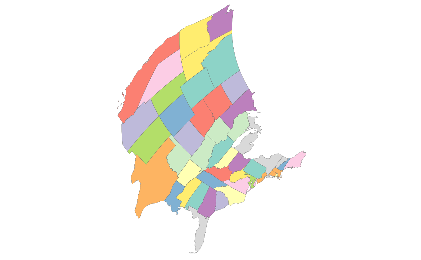
Map Find
Users can have rmap automatically search for an appropriate map using
the map_find function as follows:
library(rmap);
data = data.frame(subRegion = c("CA","FL","ID","MO","TX","WY"),
                  value = c(5,10,15,34,2,7))

map_chosen <- rmap::map_find(data)
map_chosen # Will give a dataframe for the chosen map
rmap::map(map_chosen)
Format & Themes
Layers
The map() funciton in rmap works in layers.
The central layer is created using the data provided which
fills out values for the subRegion or
lat and lon columns provided. In addition to
the central layer, users can choose an underLayer and an
overLayer to show different kinds of intersecting
boundaries or surrounding regions. The colors, border size and text
labels for each layer can be individually be modified or as a global
option. Examples of using layers are provided below for a basic
dataset.
library(rmap);

# Create data table with a few US states
data = data.frame(subRegion = c("CA","FL","ID","MO","TX","WY"),
                  value = c(5,10,15,34,2,7))

rmap::map(data) # Will choose the contiguous US map and plot this data for you as the only layer
library(rmap);

# Create data table with a few US states
data = data.frame(subRegion = c("CA","FL","ID","MO","TX","WY"),
                  value = c(5,10,15,34,2,7))
rmap::map(data,
          underLayer=rmap::mapUS49) # Will add an underlayer of the US49 map zoomed in to your data set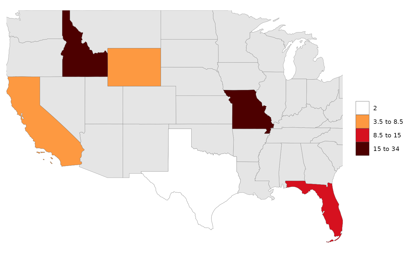
library(rmap);

# Create data table with a few US states
data = data.frame(subRegion = c("CA","FL","ID","MO","TX","WY"),
                  value = c(5,10,15,34,2,7))

rmap::map(data,
          underLayer=rmap::mapUS49,
          overLayer=rmap::mapGCAMBasinsUS49) # will add GCAM basins ontop of the previous map
Layer Colors
The line width, color and fill of each layer can be individually be modified or as a global option. Examples are provided below for a basic dataset.
# Create a basic map with no data and modify fill as well as line color and lwd.
library(rmap);
# Create data table with a few US states
mapShape = rmap::mapUS49
# Modify the line color and lwd of the base layer
rmap::map(mapShape,
          fill = "black",
          color = "white",
          lwd = 1.5) # Will adjust the borders of the different layers to highlight them.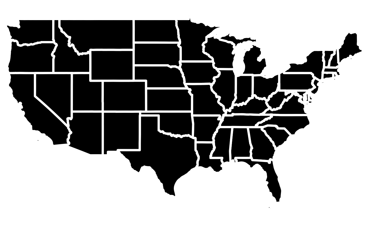
# Create a basic map with data and modify line colors and lwd.
library(rmap);
# Create data table with a few US states
data = data.frame(subRegion = c("CA","FL","ID","MO","TX","WY"),
                  value = c(5,10,15,34,2,7))
# Modify the line color and lwd of the base layer
rmap::map(data,
          color = "blue",
          lwd = 1.5) # Will adjust the borders of the different layers to highlight them.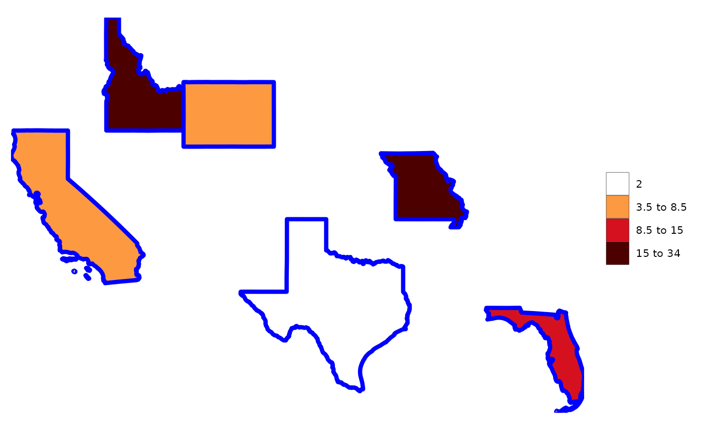
# Modify under and overlayer fill, line color and lwd.
library(rmap);
# Create data table with a few US states
data = data.frame(subRegion = c("CA","FL","ID","MO","TX","WY"),
                  value = c(5,10,15,34,2,7))

# Modify the fill and outline of the different layers
rmap::map(data,
          underLayer=rmap::mapUS49,
          underLayerFill = "black",
          underLayerColor = "green",
          underLayerLwd = 0.5,
          overLayer=rmap::mapGCAMBasinsUS49,
          overLayerColor = "red",
          overLayerLwd = 2) # Will adjust the borders of the different layers to highlight them.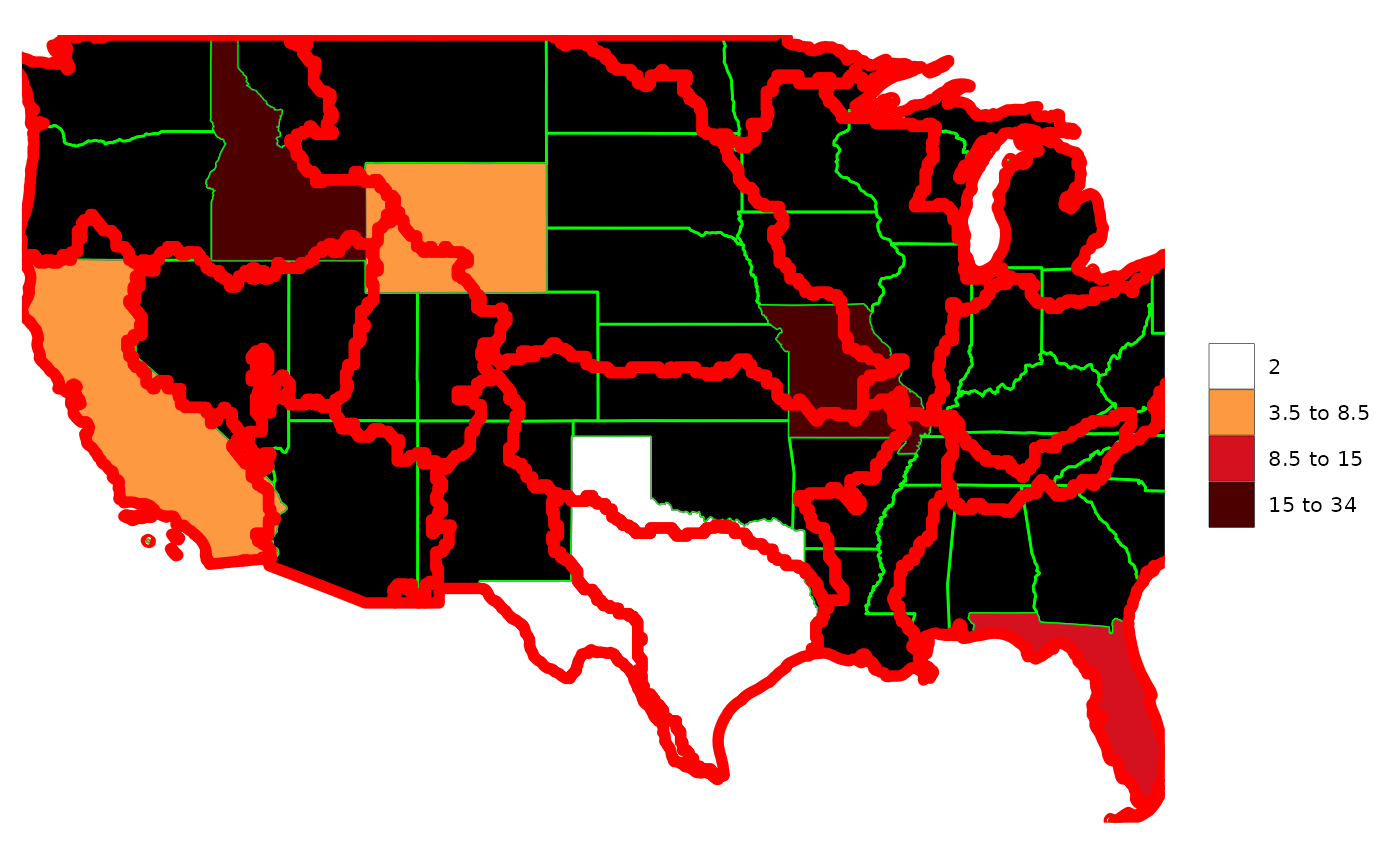
Labels
Labels can be added to the different layers of the maps as follows:
library(rmap);

# Create data table with a few US states
data = data.frame(subRegion = c("CA","FL","ID","MO","TX","WY"),
                  value = c(5,10,15,34,2,7))

# Add Blue Labels
rmap::map(data,
          labels = T,
          labelSize = 10,
          labelColor = "blue")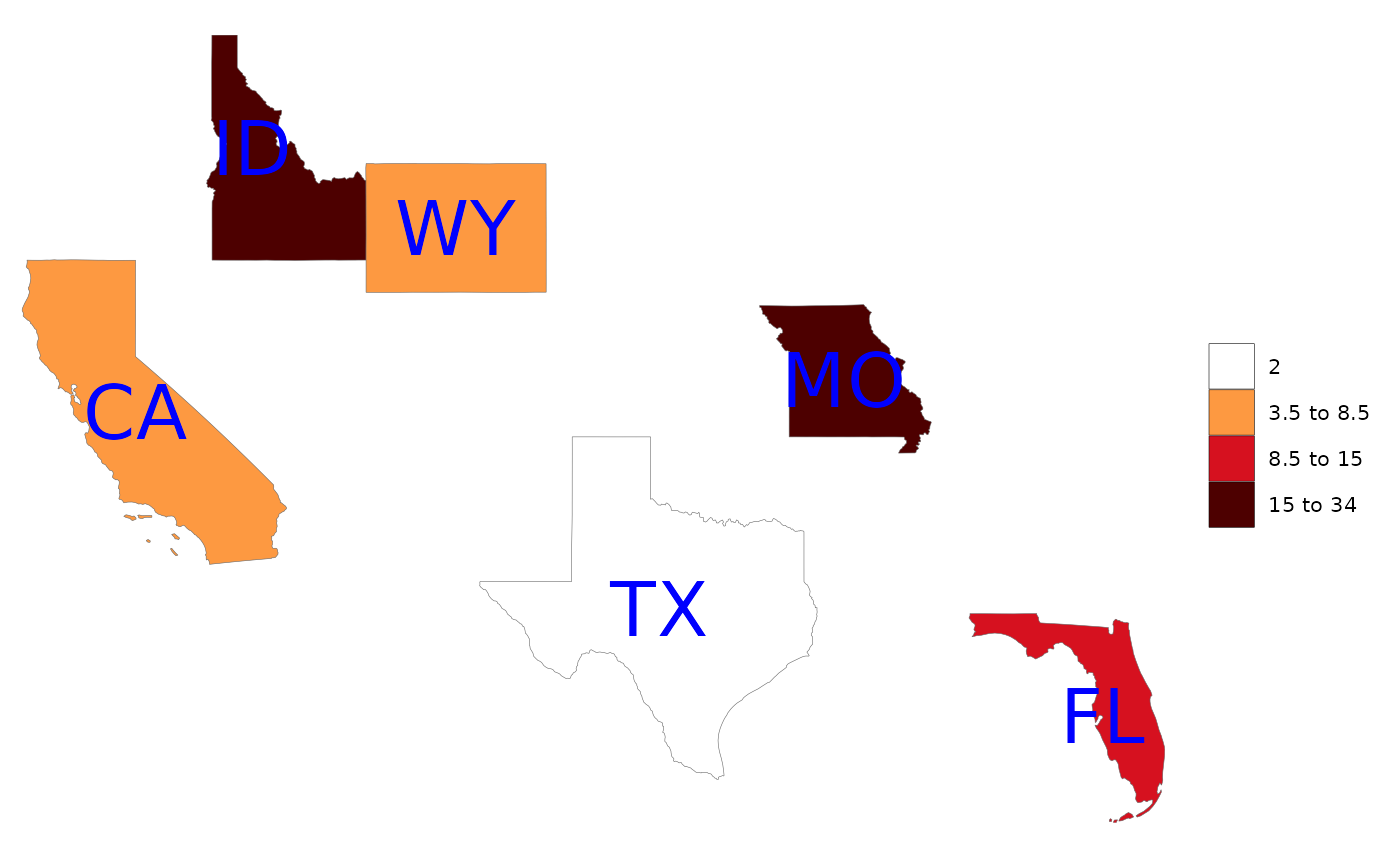
# Add labels with a transparent background box
rmap::map(data,
          labels = T,
          labelSize = 10,
          labelColor = "black",
          labelFill = "white",
          labelAlpha = 0.8,
          labelBorderSize = 1)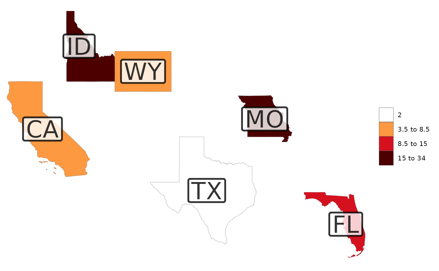
# Repel the labels out with a leader line for crowded labels
rmap::map(data=rmap::mapUS49,
          labels = T,
          labelSize = 6,
          labelColor = "black",
          labelFill = "white",
          labelAlpha = 0.8,
          labelBorderSize = 1,
          labelRepel = 1)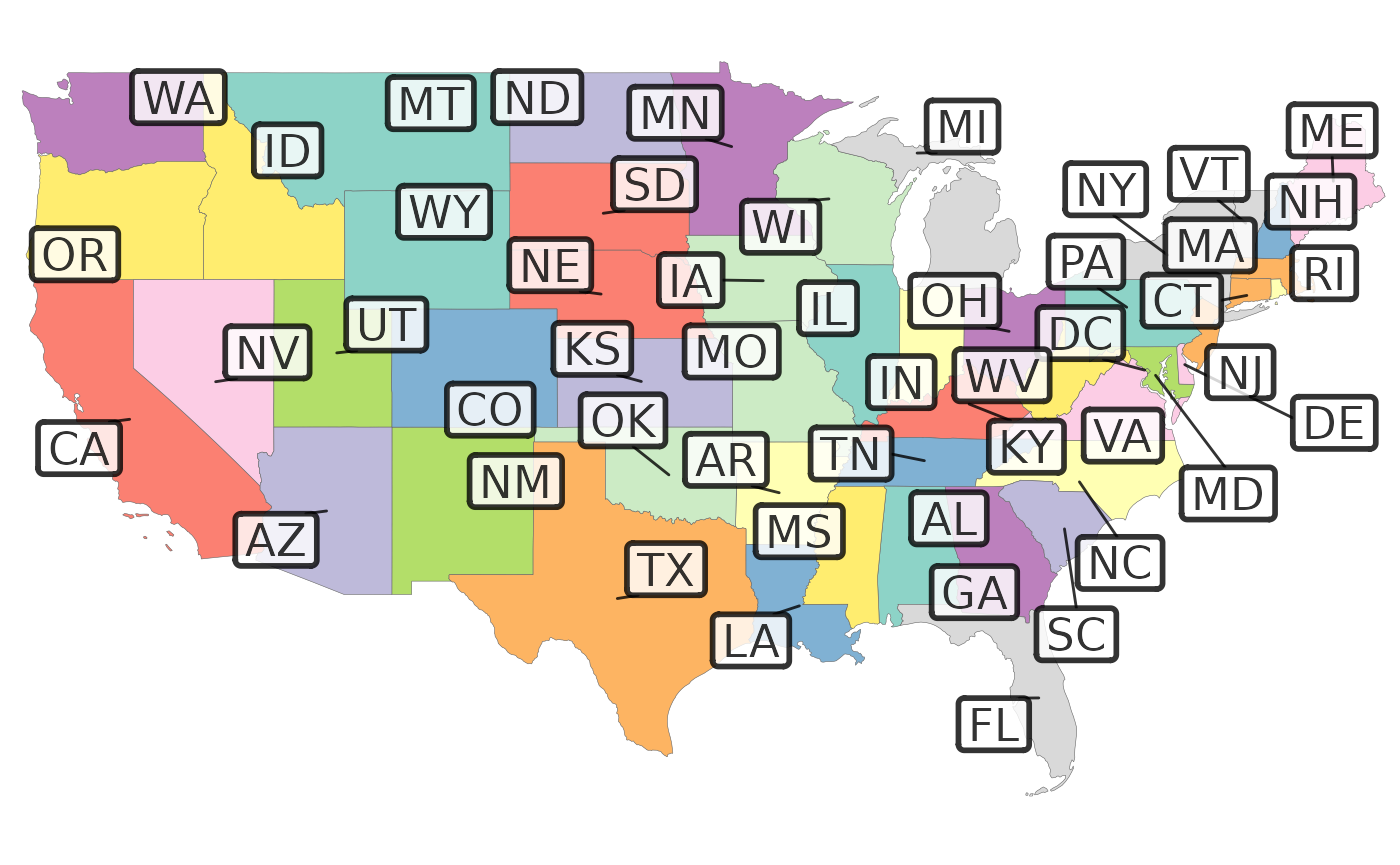
# Choose which layers to apply these label options to.
# Labels for data (labels=T), labels for underlayer (underLayerLabels=T), labels for overLayer (overLayerLabels=T)

# UnderLayer Labels Examples
rmap::map(data,
          underLayer = rmap::mapUS49,
          underLayerLabels = T)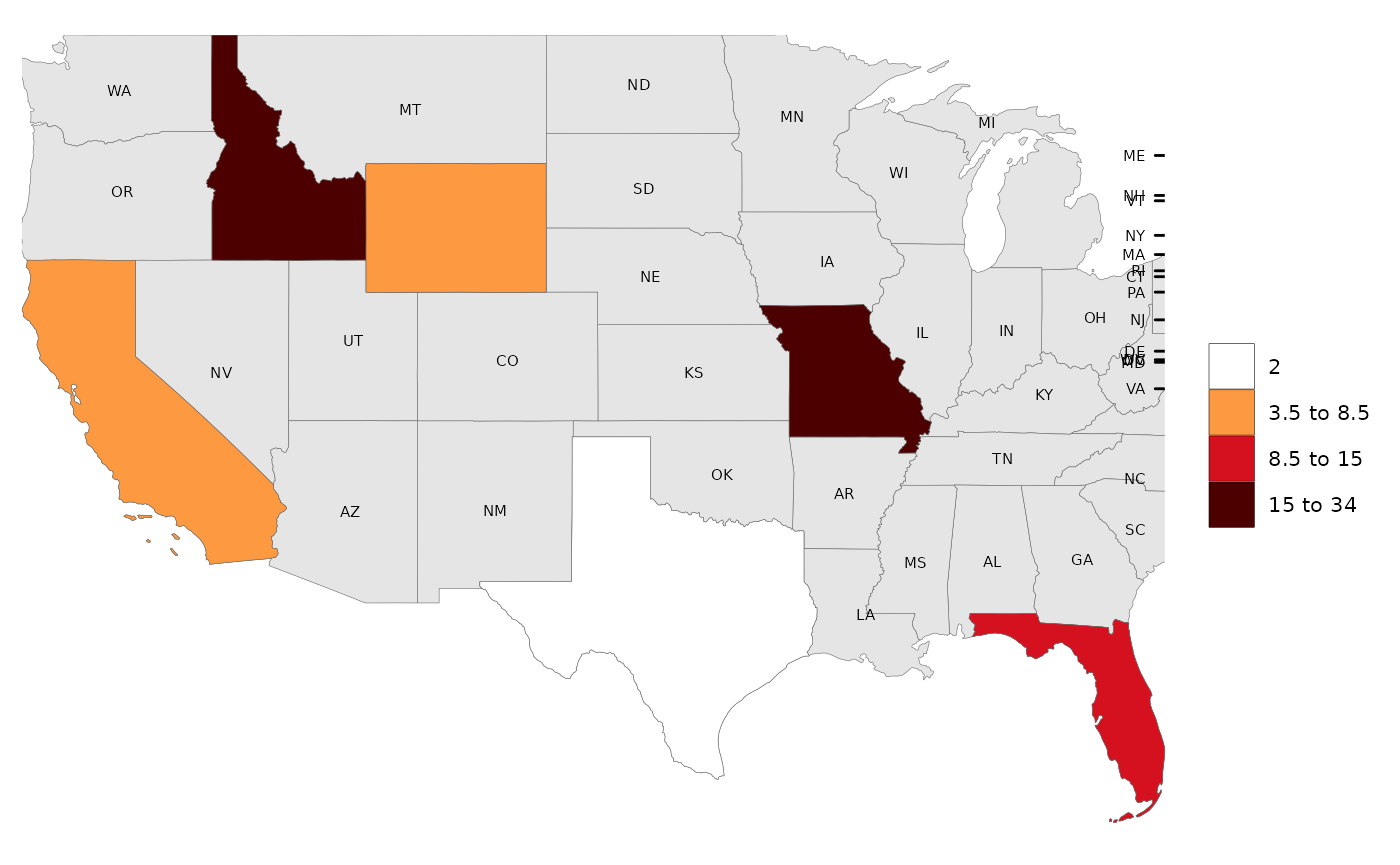
# OverLayer Examples
rmap::map(data,
          underLayer = rmap::mapUS49,
          overLayer = rmap::mapGCAMBasinsUS49,
          overLayerColor = "red",
          overLayerLabels = T,
          labelSize = 3,
          labelColor = "red",
          labelFill = "white",
          labelAlpha = 0.8,
          labelBorderSize = 0.1,
          labelRepel = 0)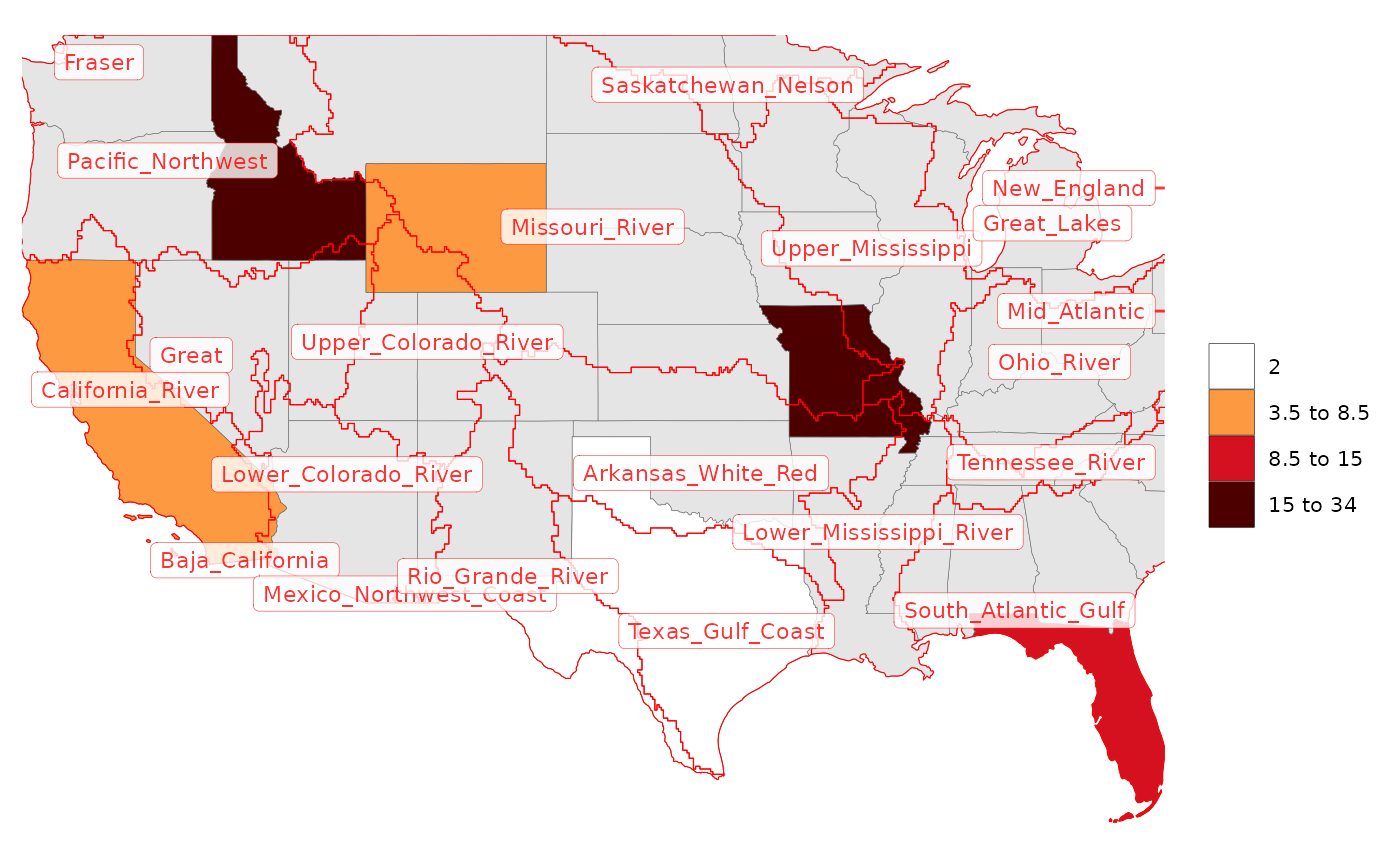
# All Labels (Not recommended as too confusing)
rmap::map(data,
          underLayer = rmap::mapUS49,
          overLayer = rmap::mapGCAMBasinsUS49,
          labels = T,
          underLayerLabels = T,
          overLayerLabels = T,
          labelSize = 2,
          labelColor = "black",
          labelFill = "white",
          labelAlpha = 0.8,
          labelBorderSize = 0.1,
          labelRepel = 1)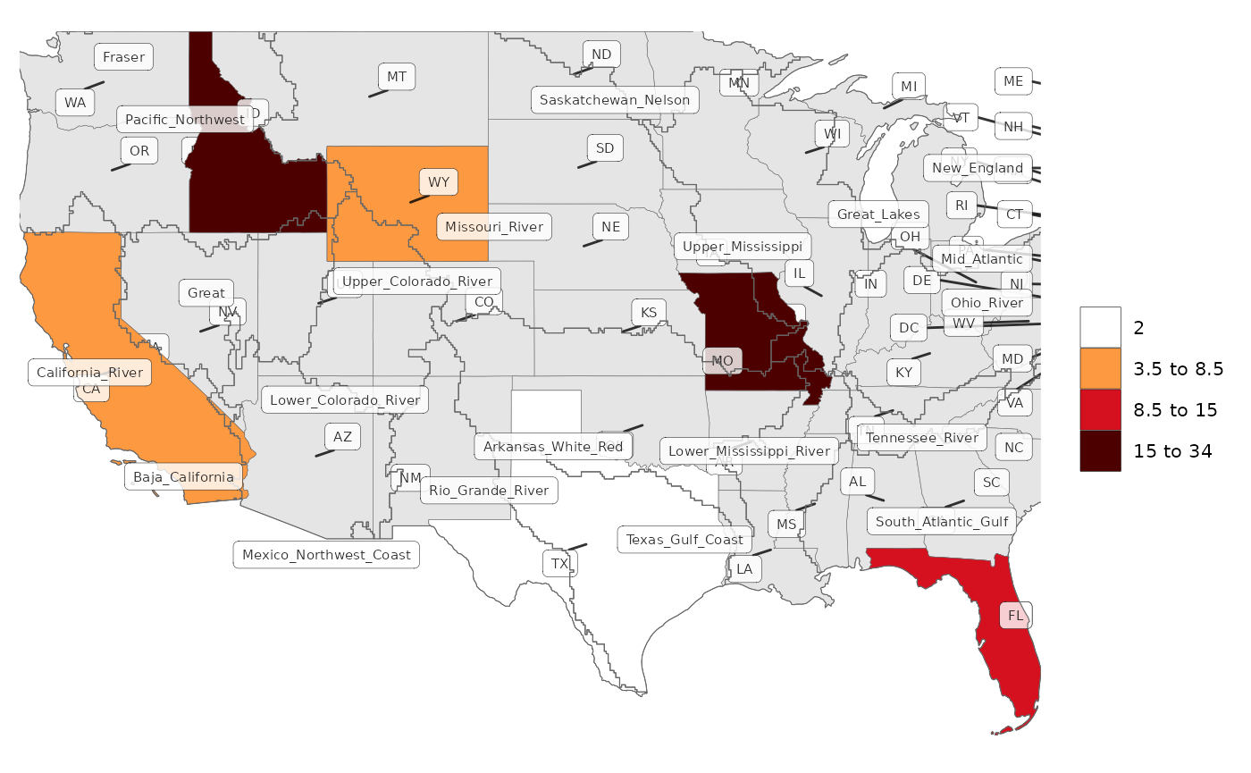
Crop
By default the maps are cropped to the extent of the subRegions
provided in the data. If the argument crop is set to
FALSE then the map will zoom to extents of the largest
layer in the map as shown below. Maps can also be cropped to the
underLayer or overLayer by setting the crop_to_underLayer
and crop_to_overLayer arguments to TRUE.
library(rmap);

# Create data table with a few US states
data = data.frame(subRegion = c("FL","ID","MO","TX","WY"),
                  value = c(10,15,34,2,7))

# Setting crop to F will zoom out to the extent of the largest layer (In this case the underLayer)
rmap::map(data,
          underLayer = rmap::mapUS49,
          underLayerLabels = T,
          labels = T,
          crop = T,
          title = "crop = T")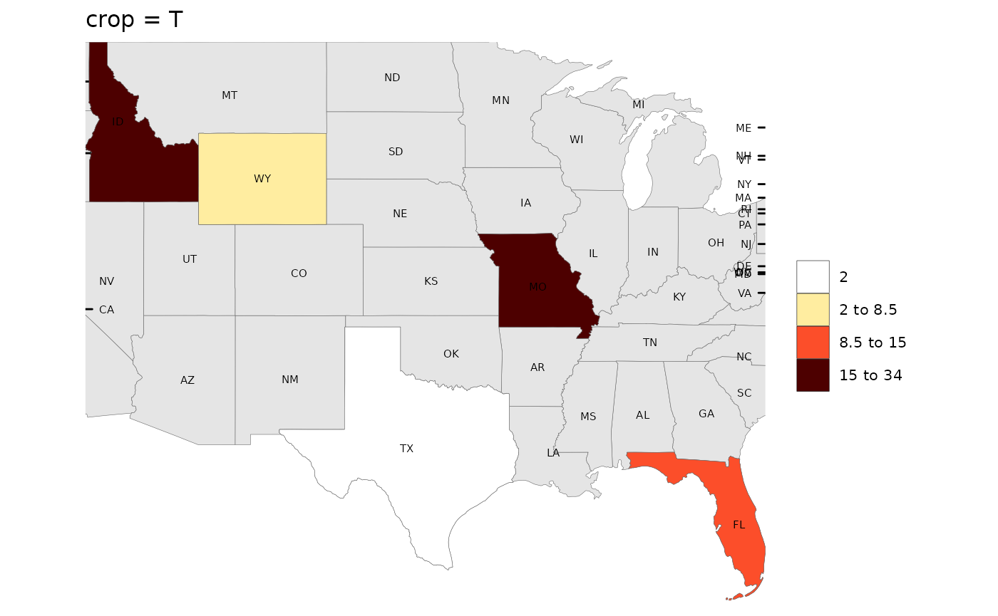
rmap::map(data,
          underLayer = rmap::mapUS49,
          underLayerLabels = T,
          labels = T,
          crop = F,
          title = "crop = F")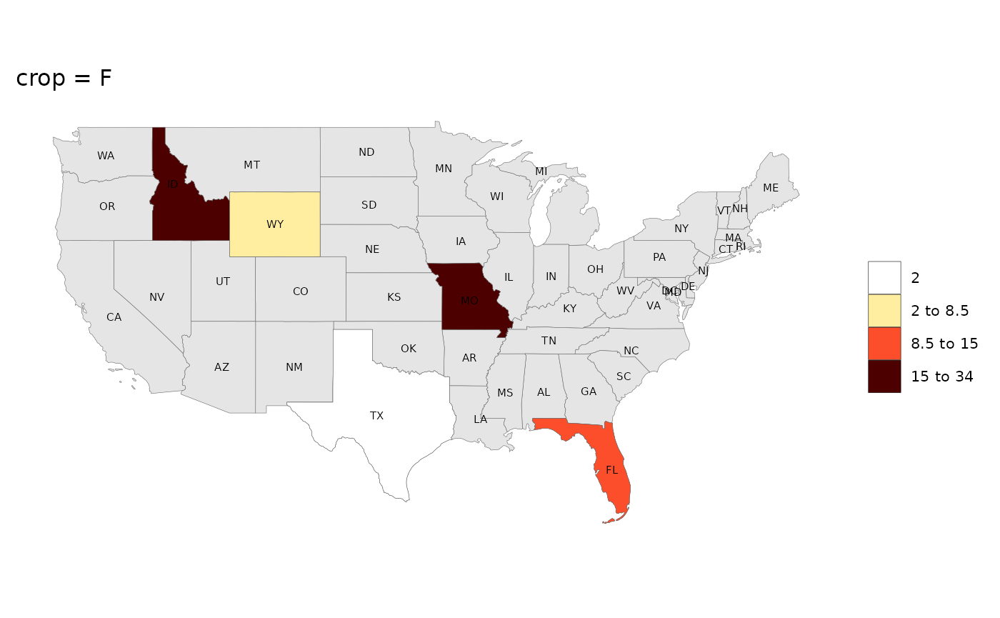
rmap::map(data,
          underLayer = rmap::mapUS49,
          overLayer = rmap::mapGCAMBasinsUS52,
          crop_to_underLayer = T,
          title = "crop_to_underLayer = T")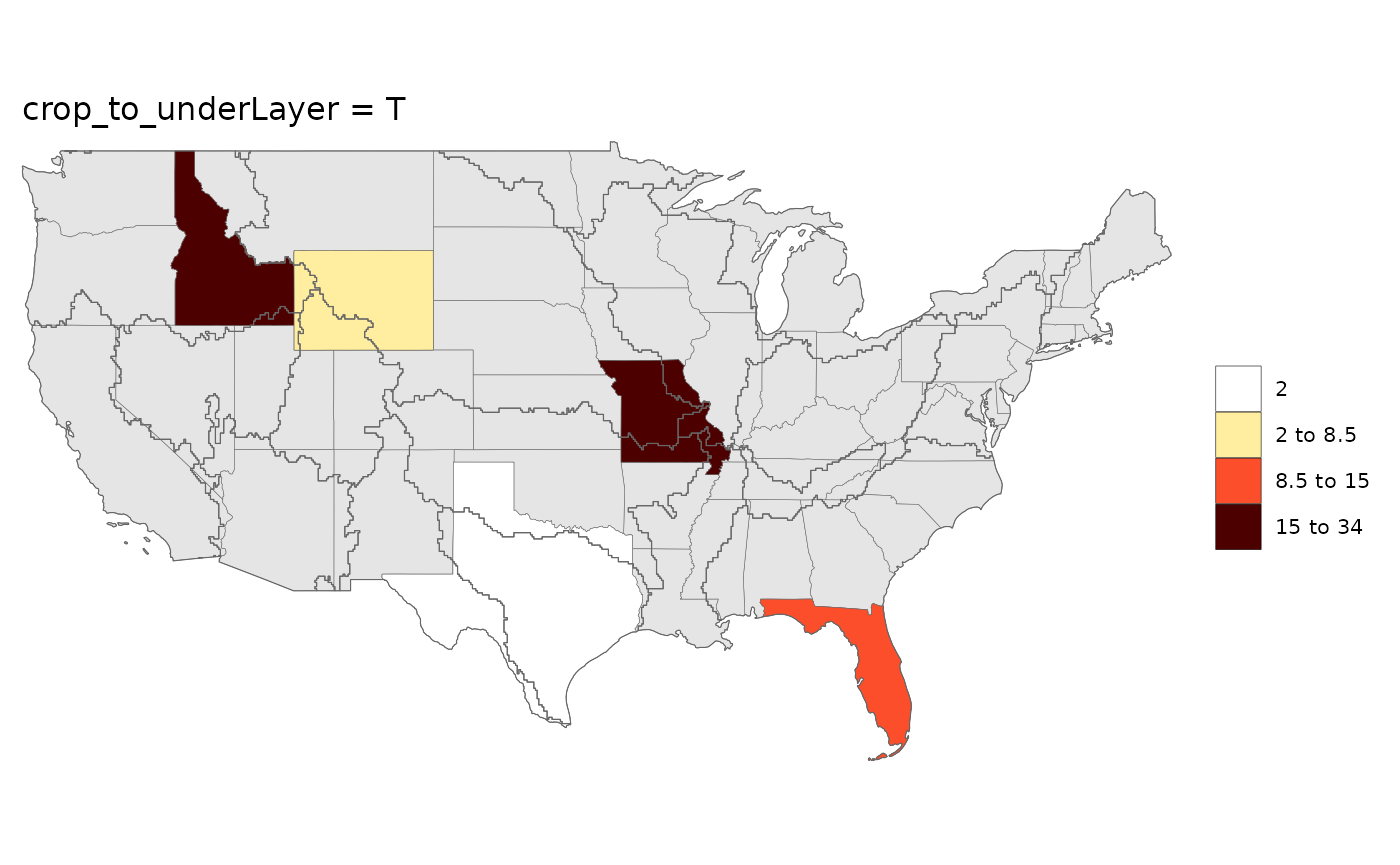
rmap::map(data,
          underLayer = rmap::mapUS49,
          overLayer = rmap::mapGCAMBasinsUS52,
          crop_to_overLayer = T,
          title = "crop_to_overLayer = T")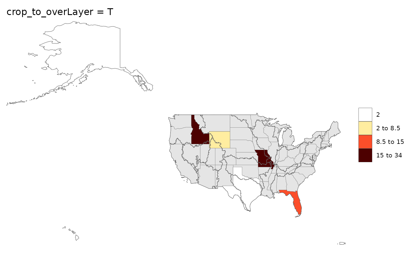
Zoom
Users can use zoom to zoom out or into a cropped map as
desired. Options are available to zoom along x only
(zoomx), along y only (zoomy) or both
(zoom).
library(rmap);

# Create data table with a few US states
data = data.frame(subRegion = c("FL","ID","MO","TX","WY"),
                  value = c(10,15,34,2,7))

# Set different zoom levels
m0 = rmap::map(data,underLayer = rmap::mapUS49,zoom = 0)
m1 = rmap::map(data,underLayer = rmap::mapUS49,zoom = 7)
m2 = rmap::map(data,underLayer = rmap::mapUS49,zoom = -10)
m3 = rmap::map(data,underLayer = rmap::mapUS49,zoomx = 3)
m4 = rmap::map(data,underLayer = rmap::mapUS49,zoomy = 4)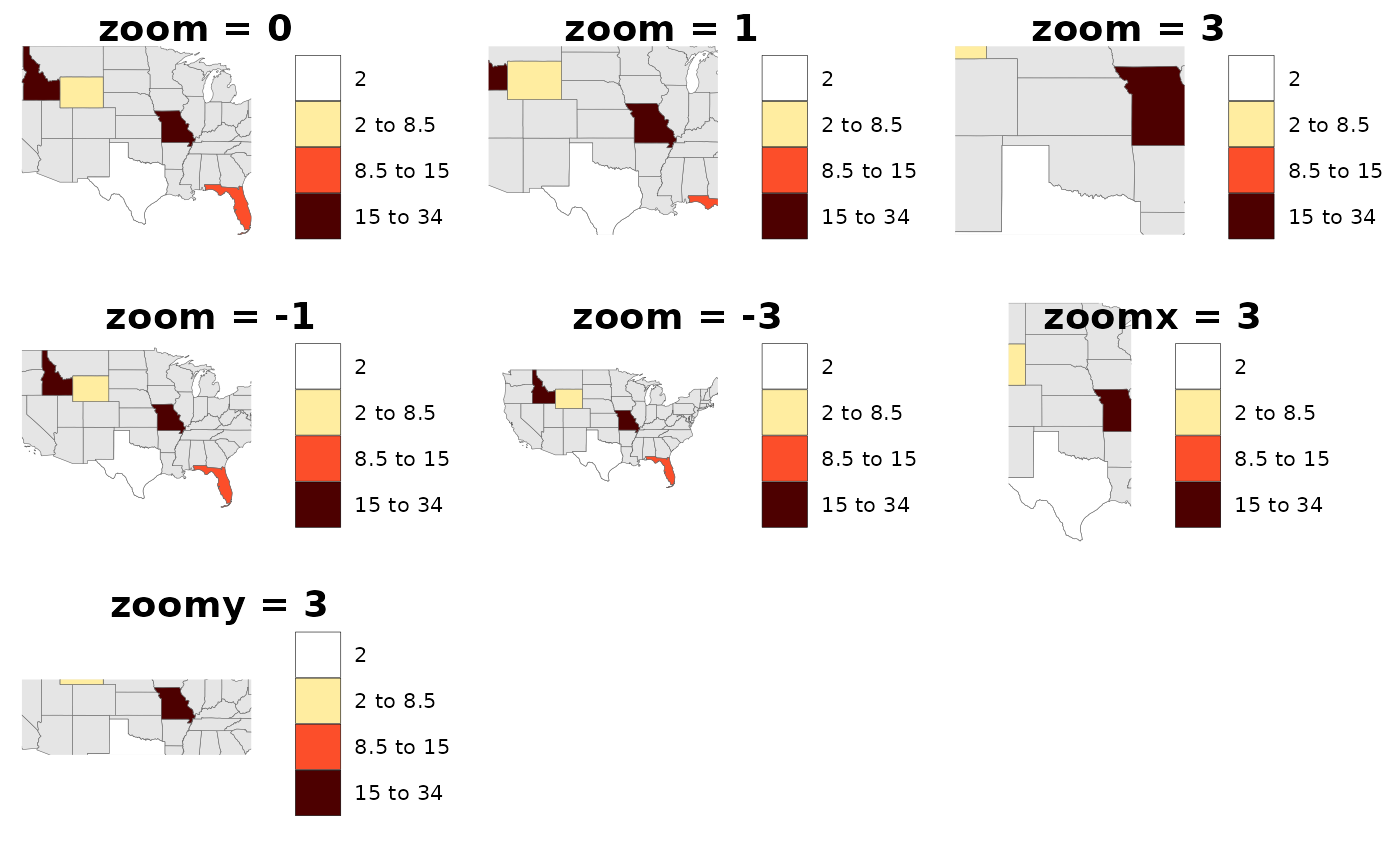
Background
While users can adjust all the elements of the map using ggplot
themes as explained in the Themes section, we have
provided a quick argument to simply add blue for oceans and a border to
the map if the background argument is set to
T. Additionally if the background argument is
set to any color such as grey10 then the map with border
will be produced with that color.
library(rmap);

# Create data table with a few US states
data = data.frame(subRegion = c("CA","FL","ID","MO","TX","WY"),
                  value = c(5,10,15,34,2,7))

# Setting background will add blue for water and a border to the map.
rmap::map(data,
          labels = T,
          underLayer = rmap::mapCountriesUS52,
          background = F,
          title = "background = F")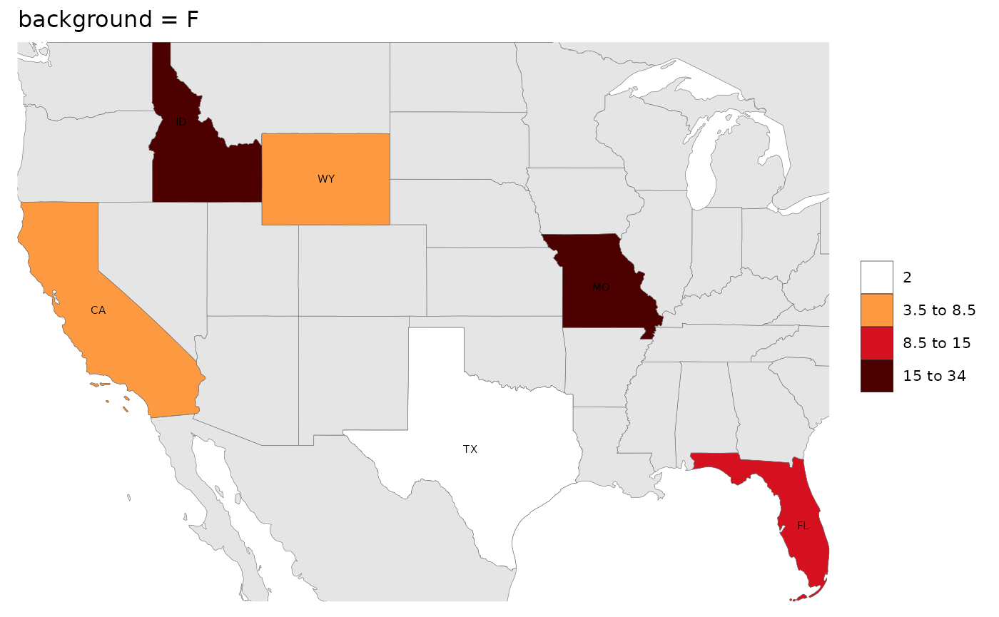
rmap::map(data,
          labels = T,
          underLayer = rmap::mapCountriesUS52,
          background = T,
          title = "background = T")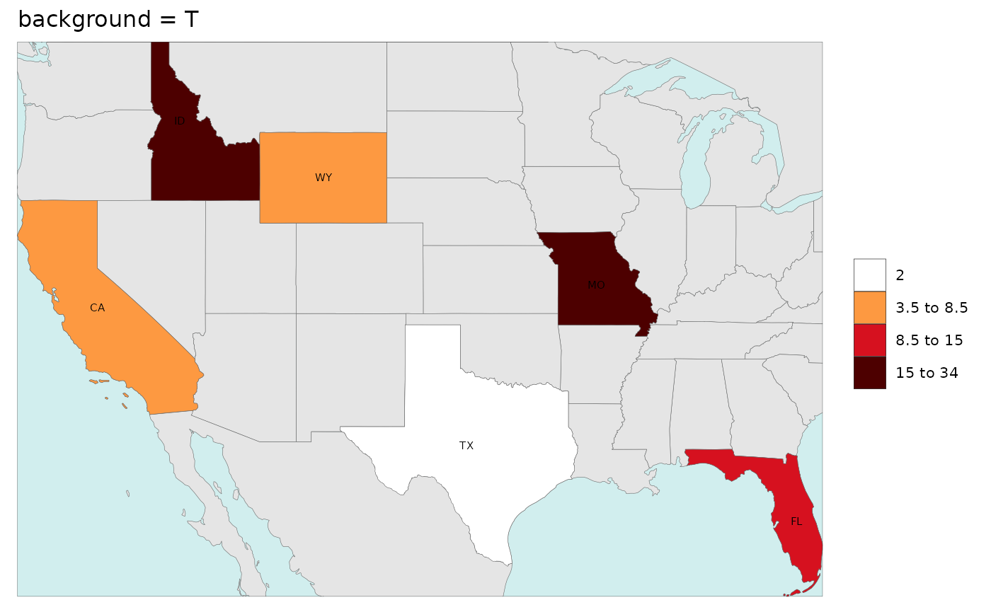
rmap::map(data,
          labels = T,
          underLayer = rmap::mapCountriesUS52,
          background = "grey10",
          title = "background = 'grey10")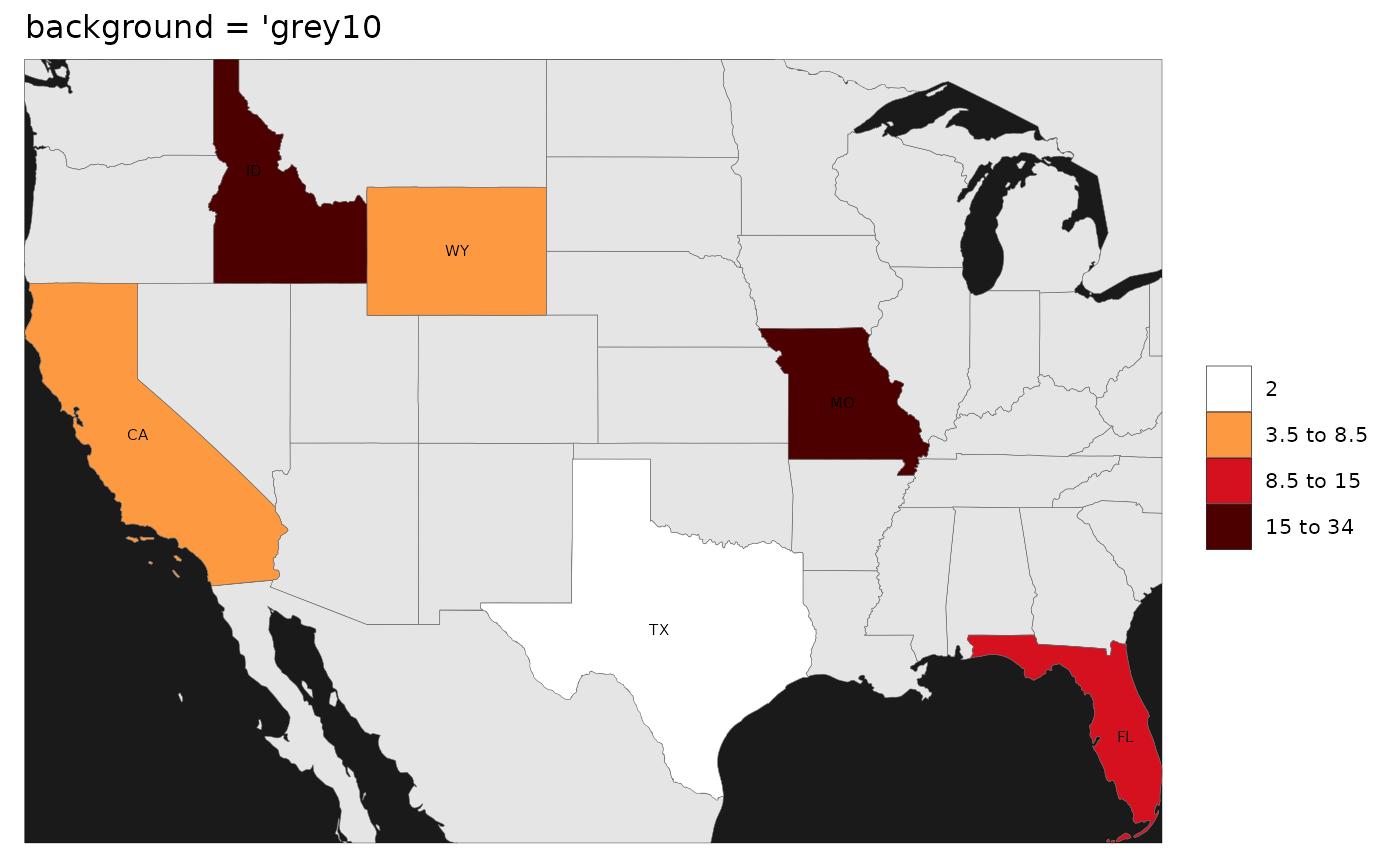
Themes
The outputs of rmap::map() is a list with
ggplot2 objects which can be modified using standard
ggplot2 themes
or by adjusting any individual component of ggplot2
elements. Some examples are shown below.
library(rmap); library(ggplot2)

# Create data table with a few US states
data = data.frame(subRegion = c("CA","FL","ID","MO","TX","WY"),
                  value = c(5,10,15,34,2,7))

# Setting m1 to the first element of the map outputs from rmap::map() with save = F to avoid printing
m1 <- rmap::map(data,
          labels = T,
          underLayer = rmap::mapCountriesUS52,
          background = T,
          show = F)

# Now Print with different ggplot elements
m1[[1]] + ggplot2::ggtitle("No Theme")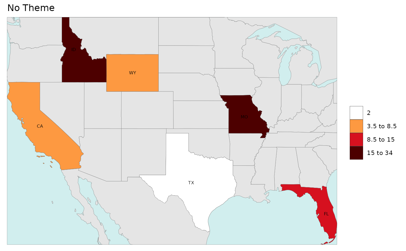
# Apply the ggplot theme_dark()
m1[[1]] +
  ggplot2::theme_dark() +
  ggplot2::ggtitle("Theme Dark") +
  ggplot2::xlab("MY X Label") +
  ggplot2::ylab("MY Y Label")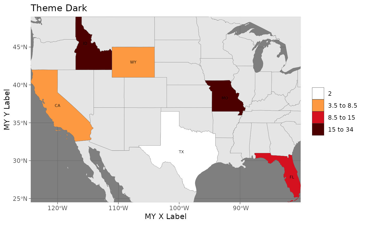
# Apply custom ggplot theme to an element
m1[[1]] +
  ggplot2::ggtitle("Themes: x label and legend position") +
  ggplot2::xlab("x label") +
  ggplot2::theme(legend.position = "bottom",
                 legend.text = element_text(size=20),
                 axis.title.x = element_text(size=20))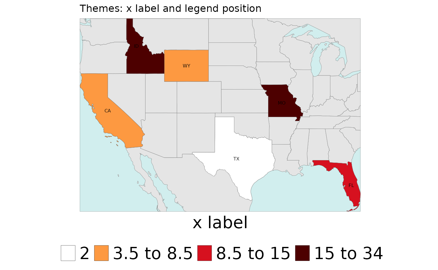
Show NA
Users have the option to showNA with a default
(gray50) or custom colors.
library(rmap)

# Create data table with a few US states
data = data.frame(subRegion = c("CA","FL","ID","MO","TX","WY"),
                  value = c(5,NA,15,34,2,7))

# Without NA
rmap::map(data,
          labels = T,
          underLayer = rmap::mapUS49,
          title = "showNA is Default (F)")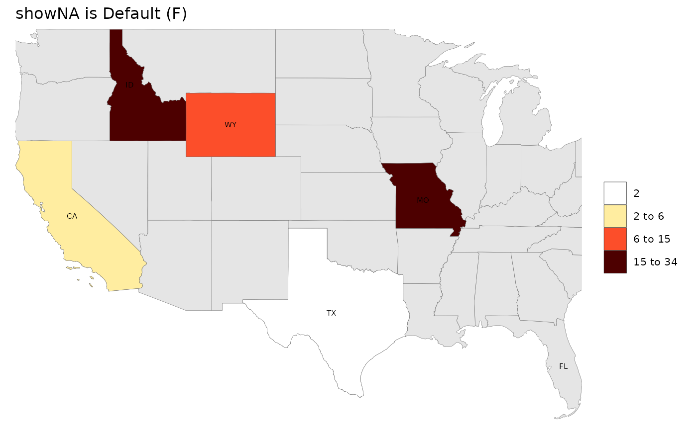
# showNA = T
rmap::map(data,
          labels = T,
          underLayer = rmap::mapUS49,
          showNA = T,
          title = "showNA = T")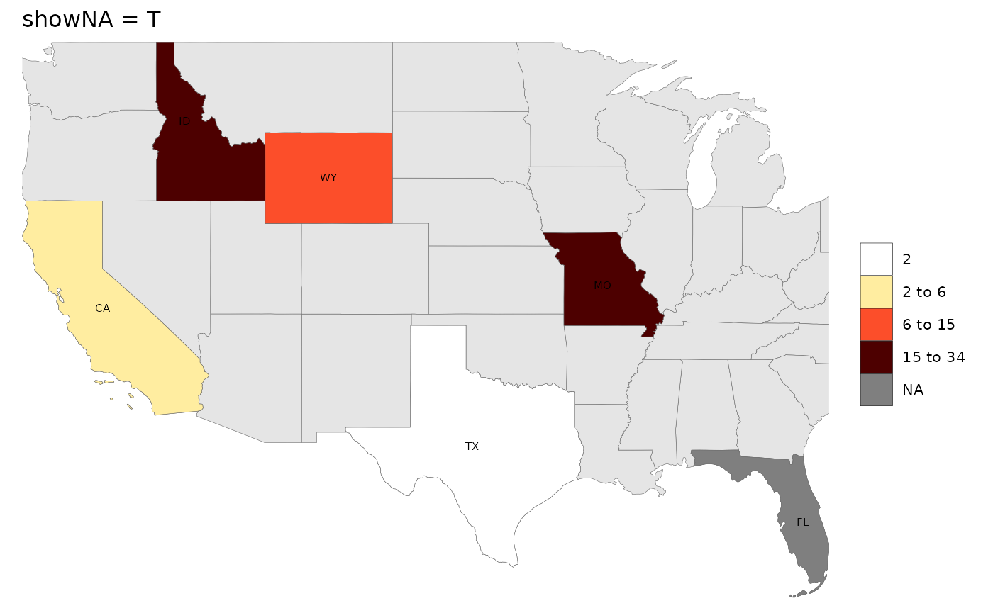
# showNA = T, colorNA = 'red'
rmap::map(data,
labels = T,
underLayer = rmap::mapUS49,
showNA = T, colorNA = 'green',
title = "showNA = T & colorNA = 'green'")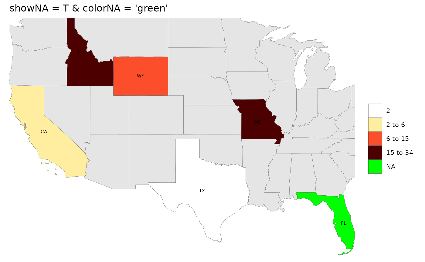 # Plot
Polygon Data
# Plot
Polygon Data
For a given data table in the correct format (see Input Format) map() will search through
the list of maps to see
if it can find the “subRegions” provided in the data and then plot the
data on the most appropriate map. Users can specify a specific map. Some
examples are provided below:
library(rmap);

# US Contiguous States
data = data.frame(subRegion = c("CA","FL","ID","MO","TX","WY"),
                  value = c(5,10,15,34,2,7))
map(data)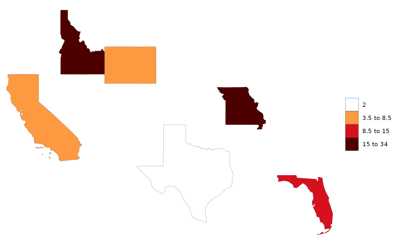
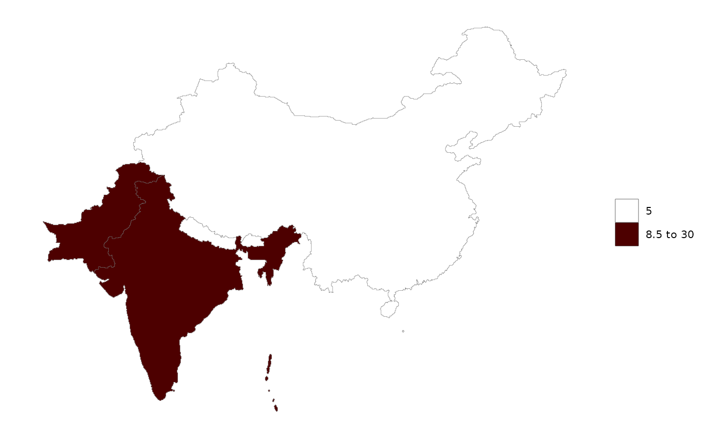
Polygon Data Select Map
Sometimes subRegions can be present on multiple maps. For example
“Colombia”, China” and “India” are all members of
rmap::mapGCAMReg32 as well as
rmap::mapCountries. If a user knows which map they want to
plot their data on they should specify the map in the shape
argument.
library(rmap)

data = data.frame(subRegion = c("China","India","Pakistan"),
                  x = c(2050,2050,2050),
                  value = c(5,12,30))

# Auto selection by rmap will choose rmap::mapCountries
rmap::map(data)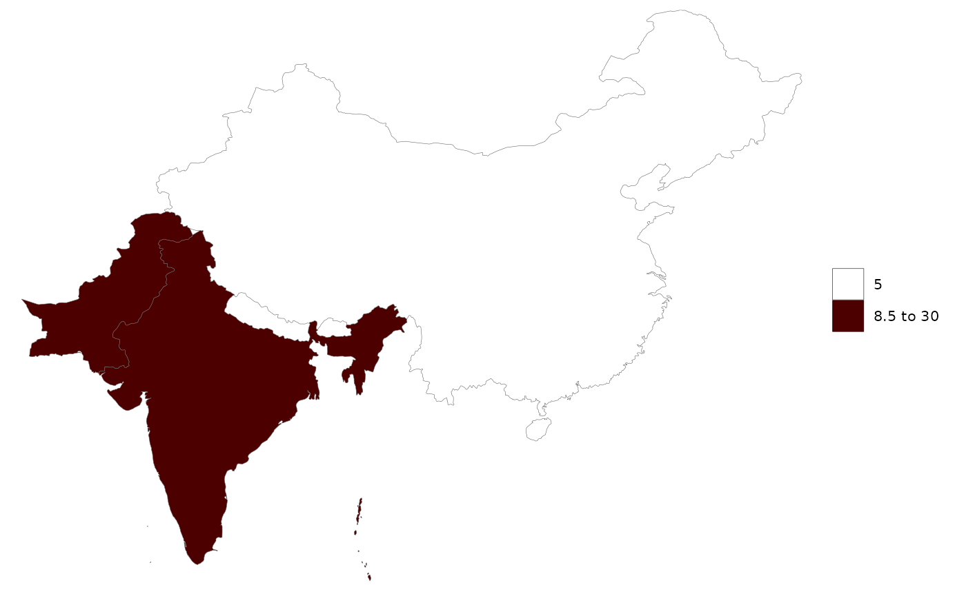
# User can specify that they want to plot this data on rmap::mapGCAMReg32
rmap::map(data,
          shape = rmap::mapGCAMReg32,
          crop = F # Because will crop to the shapes boundaries when shape is specified
          )
Plot Gridded Data
For a given data table in the correct format (see Input Format) map() will search through
the list of maps to see
if it can find the “subRegions” provided in the data and then plot the
data on the most appropriate map. Users can specify a specific map. Some
examples are provided below:
library(rmap); library(dplyr)

# Using example grid data provided in rmap
# example_gridData_GWPv4To2015
# Original data from https://sedac.ciesin.columbia.edu/data/set/gpw-v4-population-count-rev11/data-download#
# Center for International Earth Science Information Network (CIESIN) - Columbia University. 2016.
# Gridded Population of the World, Version 4 (GPWv4): Population Count. NASA Socioeconomic Data and Applications Center (SEDAC),
# Palisades, NY. DOI: http://dx.doi.org/10.7927/H4X63JVC

# Subset data
data = example_gridData_GWPv4To2015 %>%
  filter(x == 2015);
head(data)
## # A tibble: 6 × 4
## lon lat x value
## <dbl> <dbl> <chr> <dbl>
## 1 -180. -16.2 2015 895.
## 2 -180. 65.2 2015 58.6
## 3 -180. 65.8 2015 61.3
## 4 -180. 66.2 2015 70.1
## 5 -180. 66.8 2015 79.2
## 6 -180. 67.2 2015 77.6
rmap::map(data)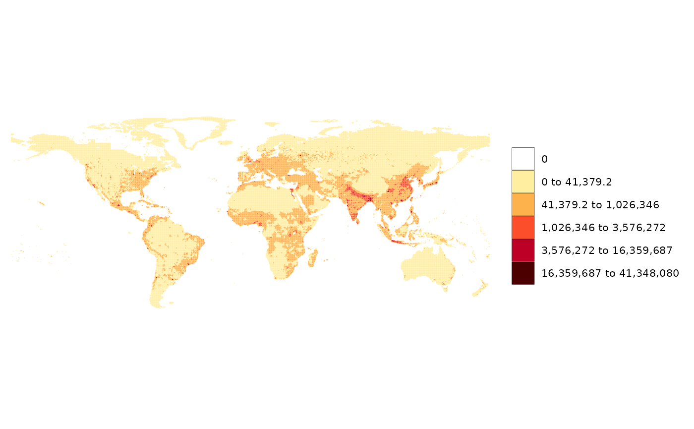
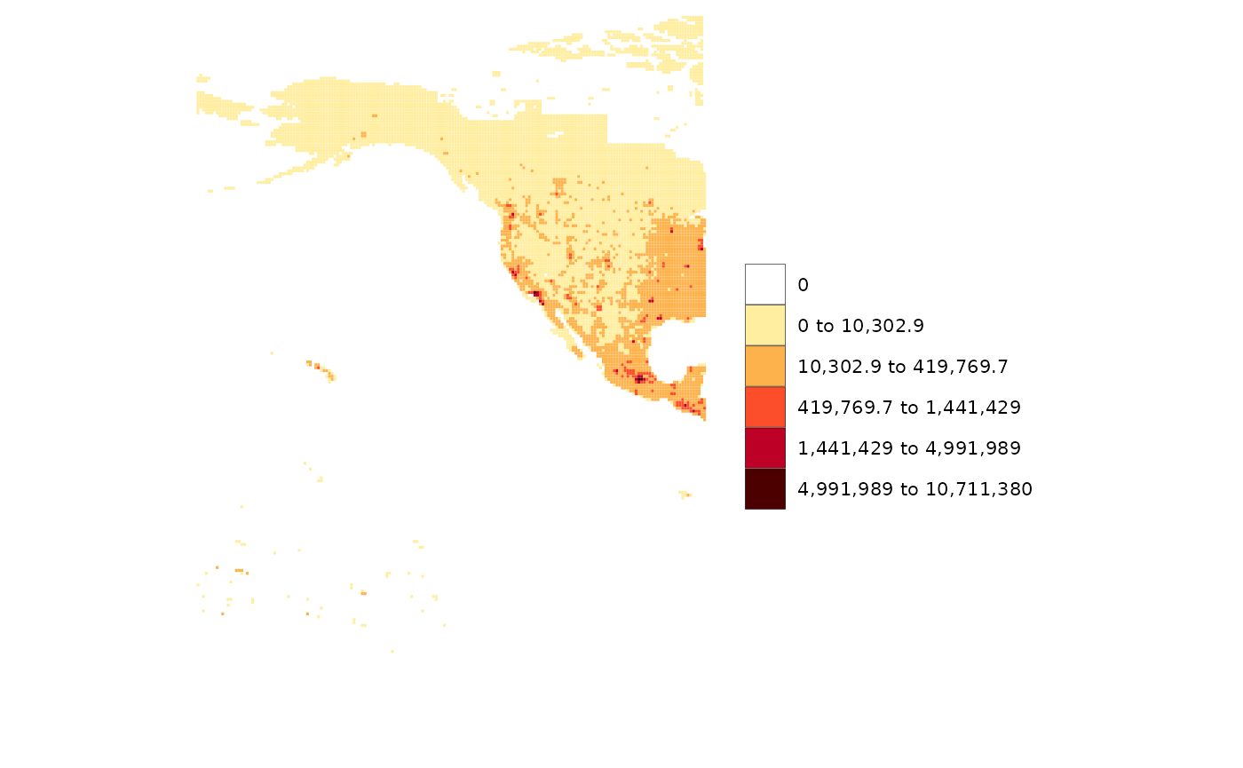
# Add an underlayer to gridded data
rmap::map(data,
          overLayer = rmap::mapCountriesUS52,
          background=T)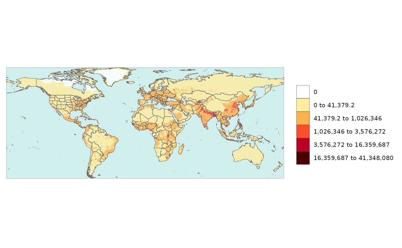
Using Custom Shapes
Users can provide custom shapefiles for their own data if needed. The example below shows how to create a custom shapefile and then plot data on it.
Subset existing shape
library(rmap)

shapeSubset <- rmap::mapStates # Read in World States shape file
shapeSubset <- shapeSubset[shapeSubset$region %in% c("Colombia"),] # Subset the shapefile to Colombia
rmap::map(shapeSubset) # View custom shape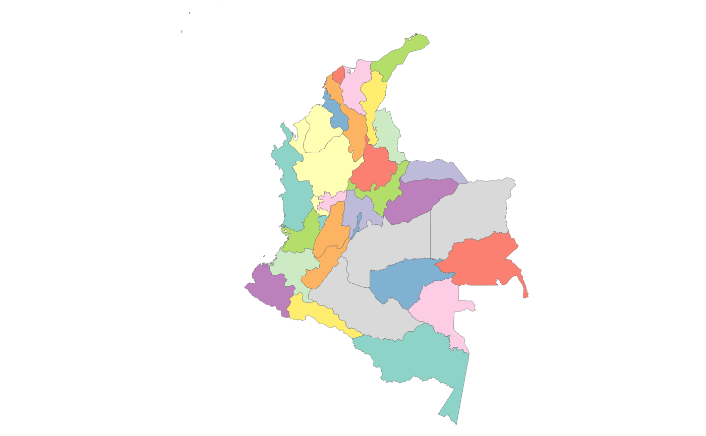
head(shapeSubset) # review data
unique(shapeSubset$subRegion) # Get a list of the unique subRegions

# Plot data on subset
data = data.frame(subRegion = c("Cauca","Valle del Cauca","Antioquia","Córdoba","Bolívar","Atlántico"),
                  x = c(2050,2050,2050,2050,2050,2050),
                  value = c(5,10,15,34,2,7))

rmap::map(data,
          shape = shapeSubset,
          underLayer = shapeSubset,
          crop=F) # Must rename the states column to 'subRegion'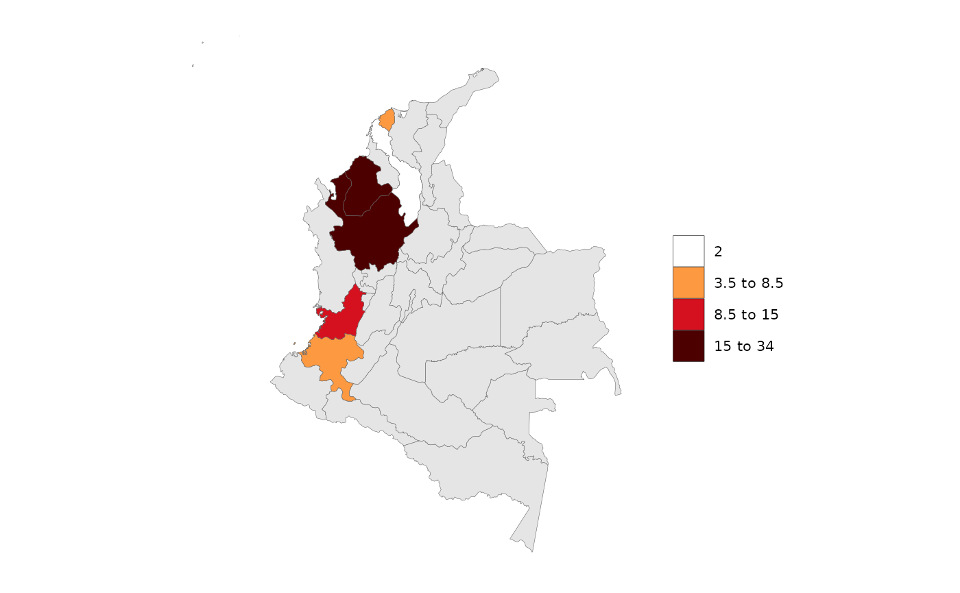
Crop a shape to another shape
For example if someone wants to analyze counties in Texas.
library(rmap); library(raster); library(sf)

shapeSubRegions <- rmap::mapUS49County
shapeCropTo <- rmap::mapUS49
shapeCropTo <- shapeCropTo[shapeCropTo$subRegion %in% c("TX"),]
shapeCrop<- sf::st_transform(shapeCropTo,sf::st_crs(shapeSubRegions))
shapeCrop <-sf::st_as_sf(raster::crop(as(shapeSubRegions,"Spatial"),as(shapeCropTo,"Spatial")))
rmap::map(shapeCrop)

# Plot data on subset
data = data.frame(subRegion = c("Wise_TX","Scurry_TX","Kendall_TX","Frio_TX","Hunt_TX","Austin_TX"),
                  value = c(5,10,15,34,2,7))
rmap::map(data,
          shape = shapeCrop,
          underLayer = shapeCrop,
          crop=F)
Save Custom Shapefile
A cropped or custom shapefile which may be much smaller in size can
be saved offline as an ESRI Shapefile for later use in
rmap or other software if desired as follows:
Read data from a Shapefile
User can read data from their own offline
ESRI Shapefile. Usually the shapefile is contained in a
single folder (e.g. custom_shape_folder) with the following
subfiles, where custom_shape will be a different name.
These kinds of files can be created in R, ArcGIS, QGIS and other
softwares (see Section Save Custom
Shapefile).
- custom_shape.dbf
- custom_shape.prj
- custom_shape.shp
- custom_shape.shx
After reading in the shapefile (e.g. as my_custom_map),
users will need to insure that it contains a subRegion
column corresponding to the features in the shape.
library(rmap); library(rgdal); library(sp)

# Assuming custom_shape files are in folder custom_shape_folder
my_custom_map = sf::st_read("path/to/custom_shape_file.shp")
head(my_custom_map)
plot(my_custom_map) # Quick view of shape
# Rename subRegion column
my_custom_map <- my_custom_map %>% dplyr::mutate(subRegion="CHOOSE_APPROPRIATE _COLUMN");

# Now a data frame with data corresponding to the custom shape regions can be created and plotted
# Generate some random data for each subRegion
data <- data.frame(subRegion=unique(my_custom_map$subRegion),
                   value = 100*runif(length(unique(my_custom_map$subRegion))));
head(data)
# And then it can be plotted using rmap and any of the built-in maps as underLayers.
rmap::map(data,
          shape=my_custom_map,
          underLayer=rmap::mapCountries,
          underLayerLabels = T)
Multi-Year-Class-Scenario-Facet
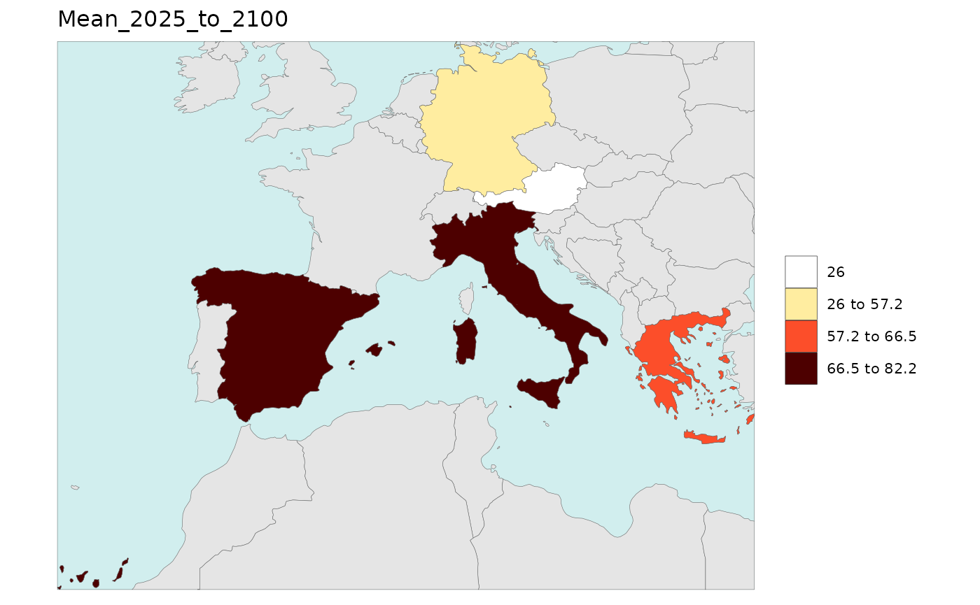
Multi-Year & Animations
Polygon Data Multi-Year
library(rmap);

data = data.frame(subRegion = c("Austria","Spain", "Italy", "Germany","Greece",
                                "Austria","Spain", "Italy", "Germany","Greece",
                                "Austria","Spain", "Italy", "Germany","Greece",
                                "Austria","Spain", "Italy", "Germany","Greece"),
                  year = c(rep(2025,5),
                               rep(2050,5),
                               rep(2075,5),
                               rep(2100,5)),
                  value = c(32, 38, 54, 63, 24,
                            37, 53, 23, 12, 45,
                            23, 99, 102, 85, 75,
                            12, 76, 150, 64, 90))

rmap::map(data = data,
          underLayer = rmap::mapCountries,
          ncol=4,
          background = T)

# NOTE: Animation files are only saved to file and not as a direct output of the rmap::map() function.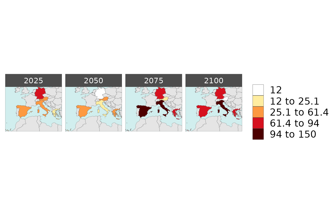
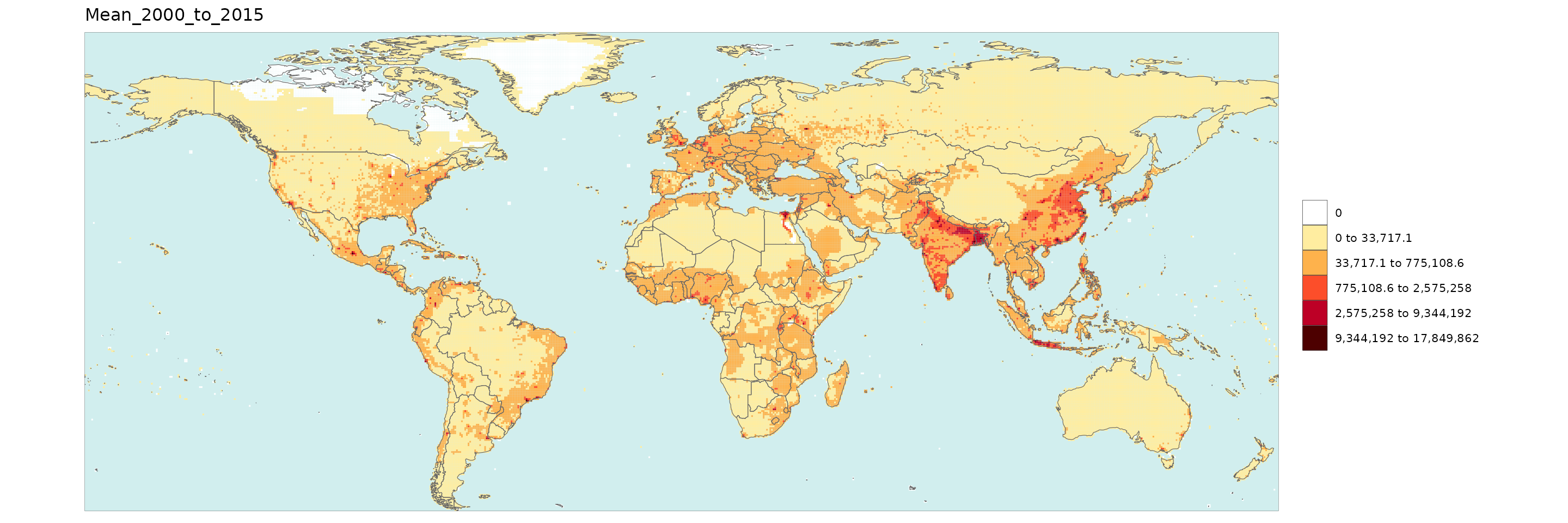
Gridded Data Multi-Year
## # A tibble: 6 × 4
##     lon   lat x     value
##   <dbl> <dbl> <chr> <dbl>
## 1 -180. -16.2 2000   786.
## 2 -180.  65.2 2000   120.
## 3 -180.  65.8 2000   126.
## 4 -180.  66.2 2000   144.
## 5 -180.  66.8 2000   163.
## 6 -180.  67.2 2000   159.
library(rmap);
rmap::map(data = data,
          overLayer = rmap::mapCountries,
          background = T, width = 15, height =15)

# NOTE: Animation files are only saved to file and not as a direct output of the rmap::map() function.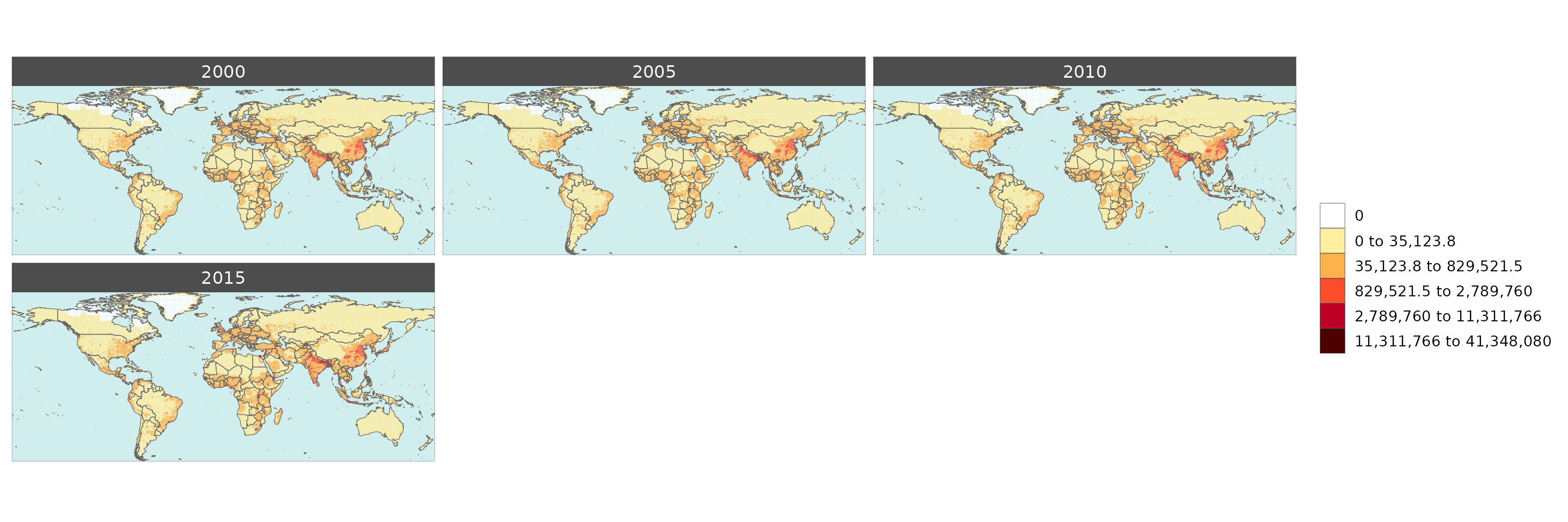
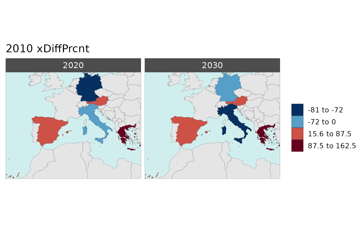
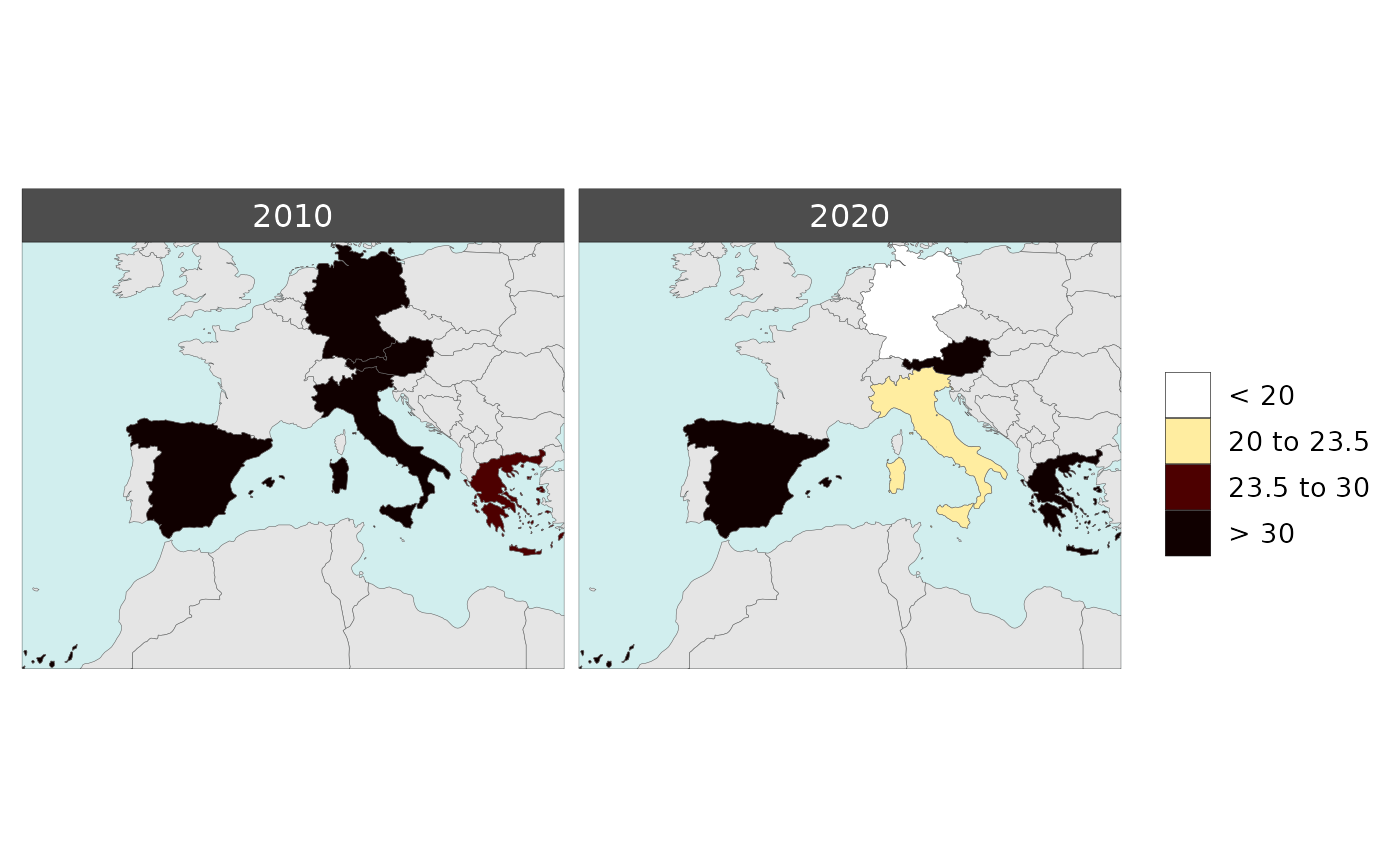
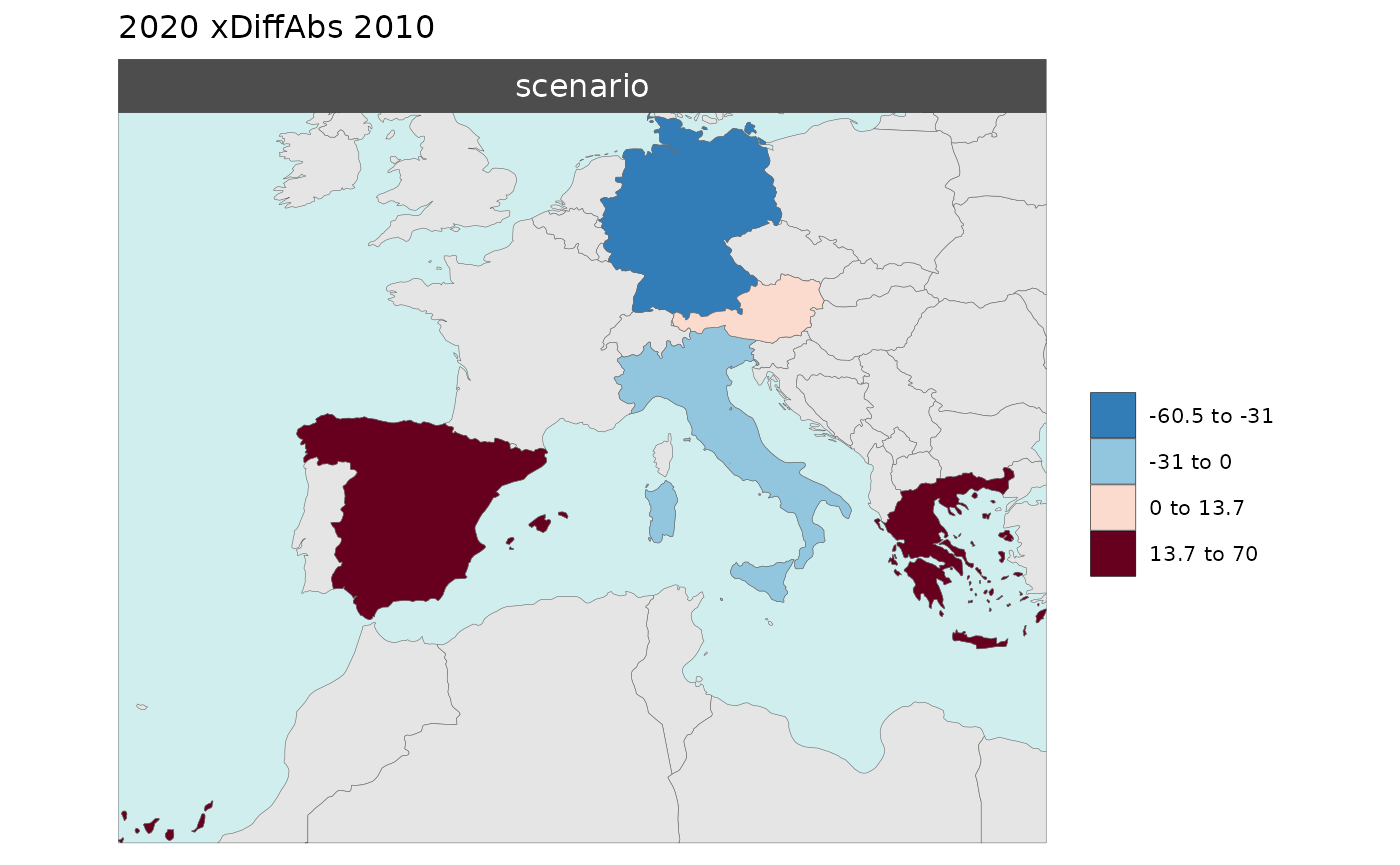
Multi-Year Diff plots
When multiple years are present in the data, assigning an
xRef and xDiff will result in
rmap::map() to calculate the absolute and percentage
difference between the chosen xref year and
xDiff years and store them in corresponding folders.
Polygon Data Multi-Year Diff
library(rmap);

data = data.frame(subRegion = c("Austria","Spain", "Italy", "Germany","Greece",
                                "Austria","Spain", "Italy", "Germany","Greece",
                                "Austria","Spain", "Italy", "Germany","Greece"),
                  year = c(rep(2010,5),rep(2020,5),rep(2030,5)),
                  value = c(32, 38, 54, 63, 24,
                            37, 53, 23, 12, 45,
                            40, 45, 12, 50, 63))

mapx <- rmap::map(data = data,
          background = T,
          underLayer = rmap::mapCountries,
          xRef = 2010,
          xDiff = c(2020,2030))

mapx$map_param_KMEANS_xDiffAbs
mapx$map_param_KMEANS_xDiffPrcnt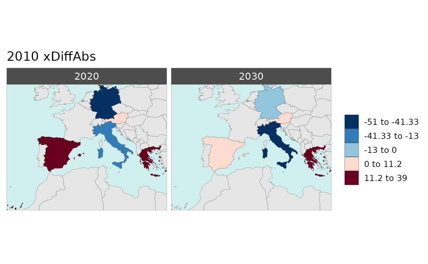
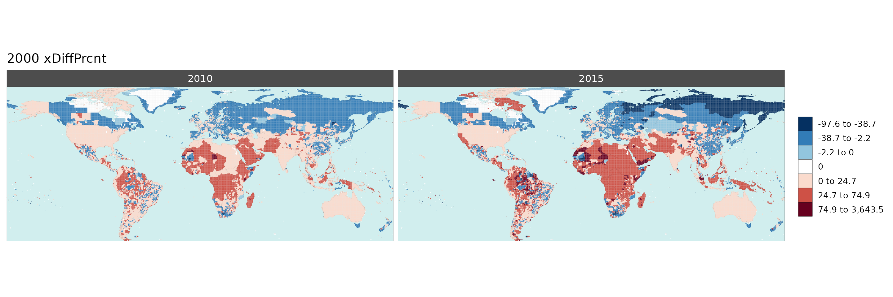
Gridded Data Multi-Year Diff
library(rmap);

data = example_gridData_GWPv4To2015
mapx <- rmap::map(data = data,
          background = T,
          underLayer = rmap::mapCountries,
          xRef = 2000,
          xDiff = c(2010,2015), diffOnly = T, width = 15, height =15)

mapx$map_param_KMEANS_xDiffAbs
mapx$map_param_KMEANS_xDiffPrcnt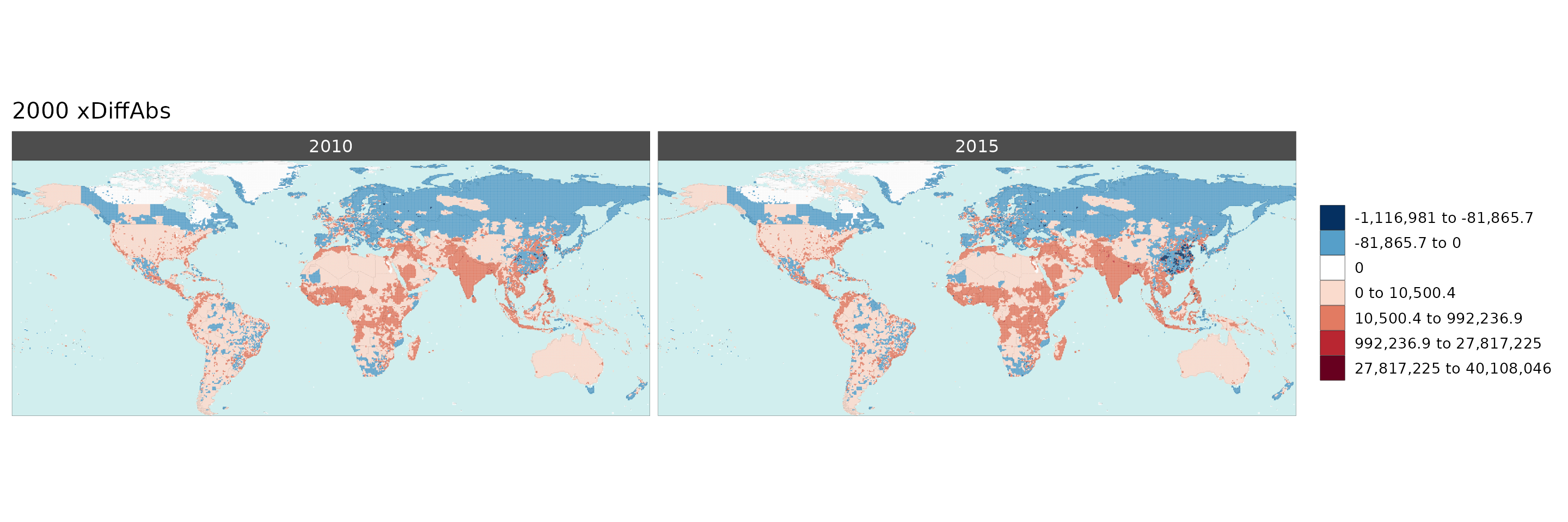
Multi-Class
Polygon Data Multi-Class
library(rmap);

data = data.frame(subRegion = c("Austria","Spain", "Italy", "Germany","Greece",
                                "Austria","Spain", "Italy", "Germany","Greece",
                                "Austria","Spain", "Italy", "Germany","Greece",
                                "Austria","Spain", "Italy", "Germany","Greece"),
                  class = c(rep("municipal",5),
                               rep("industry",5),
                               rep("agriculture",5),
                               rep("transport",5)),
                  value = c(32, 38, 54, 63, 24,
                            37, 53, 23, 12, 45,
                            23, 99, 102, 85, 75,
                            12, 76, 150, 64, 90))
rmap::map(data = data,
          underLayer = rmap::mapCountries,
          background = T )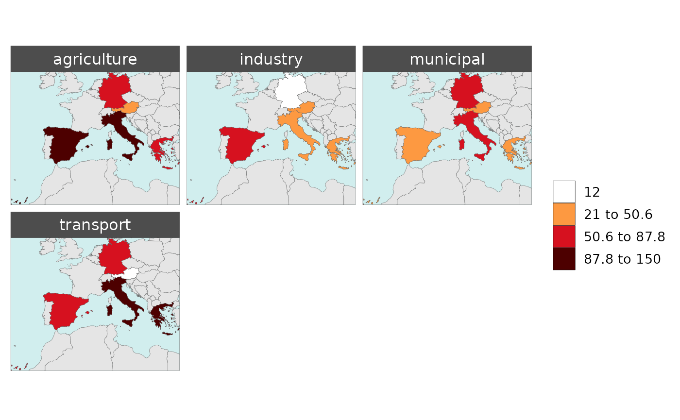
Gridded Data Multi-Class
library(rmap);library(dplyr)

# Change the years in the gridded data to classes
data = example_gridData_GWPv4To2015 %>%
  dplyr::rename(class=x) %>%
  dplyr::mutate(class = dplyr::case_when(
    class == "2000" ~ "municipal",
    class == "2005" ~ "agriculture",
    class == "2010" ~ "water",
    class == "2015" ~ "other",
    TRUE ~ class
  ))

rmap::map(data = data,
          overLayer = rmap::mapCountries,
          background = T,
          ncol = 2, width = 15, height =15)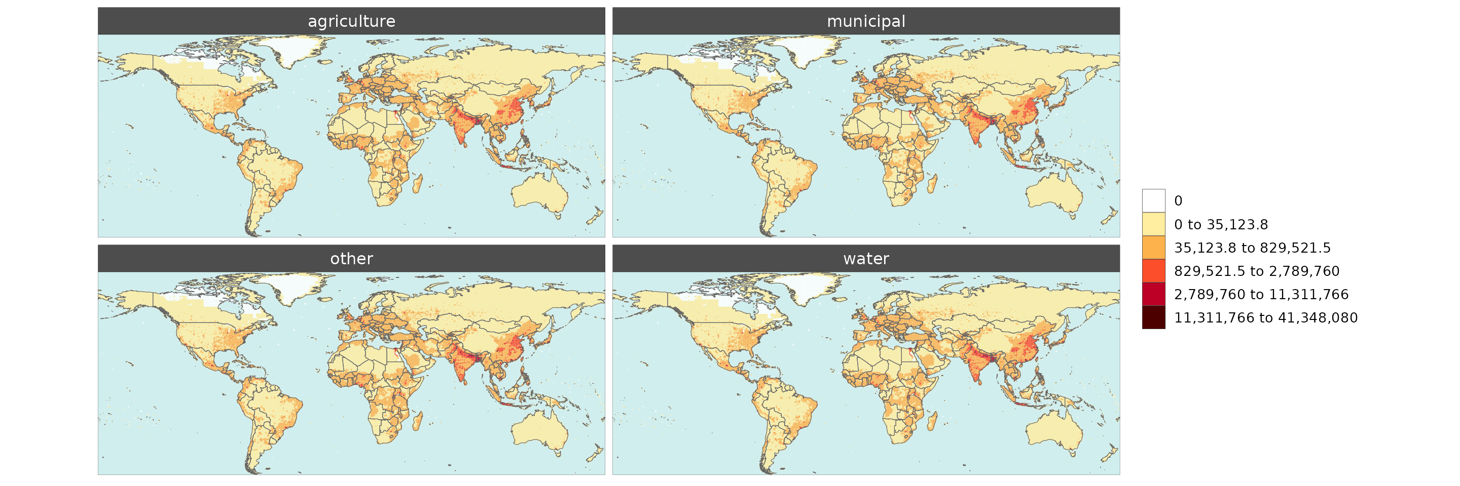
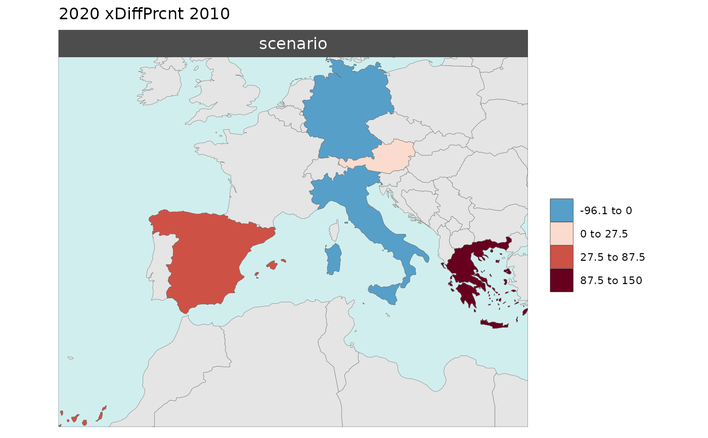
Multi-Scenario
With multiple scenarios present an additional folder and maps for combined scenarios are produced.
Polygon Data Multi-Scenario
library(rmap);

data = data.frame(subRegion = c("Austria","Spain", "Italy", "Germany","Greece",
                                "Austria","Spain", "Italy", "Germany","Greece",
                                "Austria","Spain", "Italy", "Germany","Greece"),
                  scenario = c("scen1","scen1","scen1","scen1","scen1",
                               "scen2","scen2","scen2","scen2","scen2",
                               "scen3","scen3","scen3","scen3","scen3"),
                  year = rep(2010,15),
                  value = c(32, 38, 54, 63, 24,
                            37, 53, 23, 12, 45,
                            40, 44, 12, 30, 99))

mapx <- rmap::map(data = data,
          underLayer = rmap::mapCountries,
          background = T)

mapx$map_param_KMEANS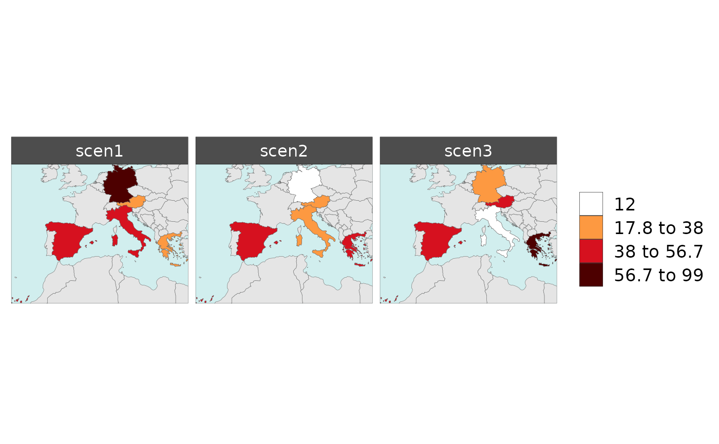
Customize Order of Scenarios
library(rmap);

data = data.frame(subRegion = c("Austria","Spain", "Italy", "Germany","Greece",
                                "Austria","Spain", "Italy", "Germany","Greece",
                                "Austria","Spain", "Italy", "Germany","Greece"),
                  scenario = c("scen1","scen1","scen1","scen1","scen1",
                               "scen2","scen2","scen2","scen2","scen2",
                               "scen3","scen3","scen3","scen3","scen3"),
                  year = rep(2010,15),
                  value = c(32, 38, 54, 63, 24,
                            37, 53, 23, 12, 45,
                            40, 44, 12, 30, 99))

# Reorder your scenarios
data = data %>%
  dplyr::mutate(scenario = factor(scenario, levels = c("scen1","scen3","scen2")))

mapx <- rmap::map(data = data,
          underLayer = rmap::mapCountries,
          background = T)

mapx$map_param_KMEANS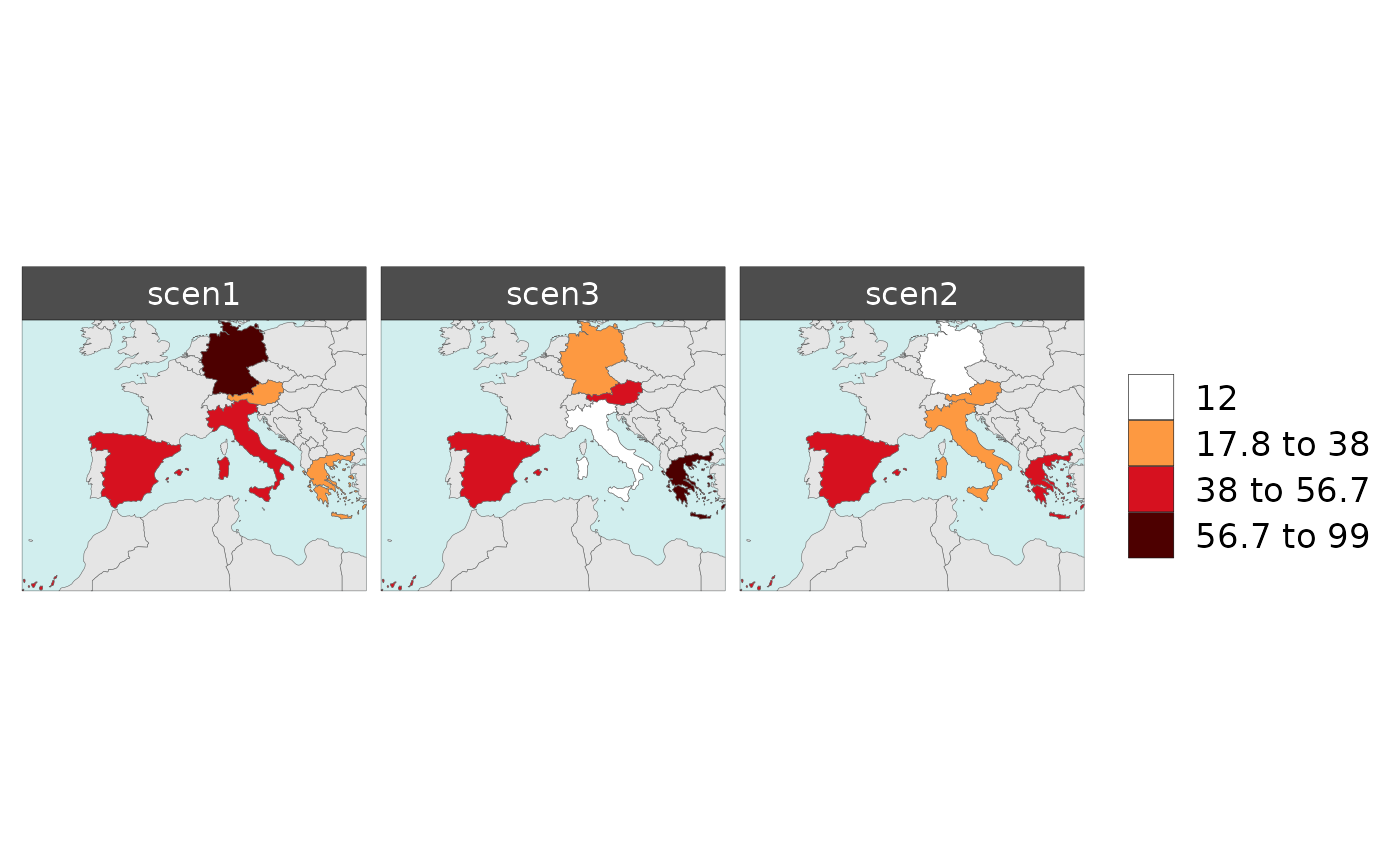
Gridded Data Multi-Scenario
library(rmap);

# Change the years in the example gridded data to scenarios
data = example_gridData_GWPv4To2015 %>%
  dplyr::filter(x %in% c("2000","2005","2010")) %>%
  dplyr::rename(scenario=x) %>%
  dplyr::mutate(scenario = dplyr::case_when(
    scenario == "2000" ~ "scenario1",
    scenario == "2005" ~ "scenario2",
    scenario == "2010" ~ "scenario3",
    TRUE ~ scenario))

mapx <- rmap::map(data = data,
          underLayer = rmap::mapCountries,
          background = T,
          ncol = 1, width = 15, height =15)

mapx$map_param_KMEANS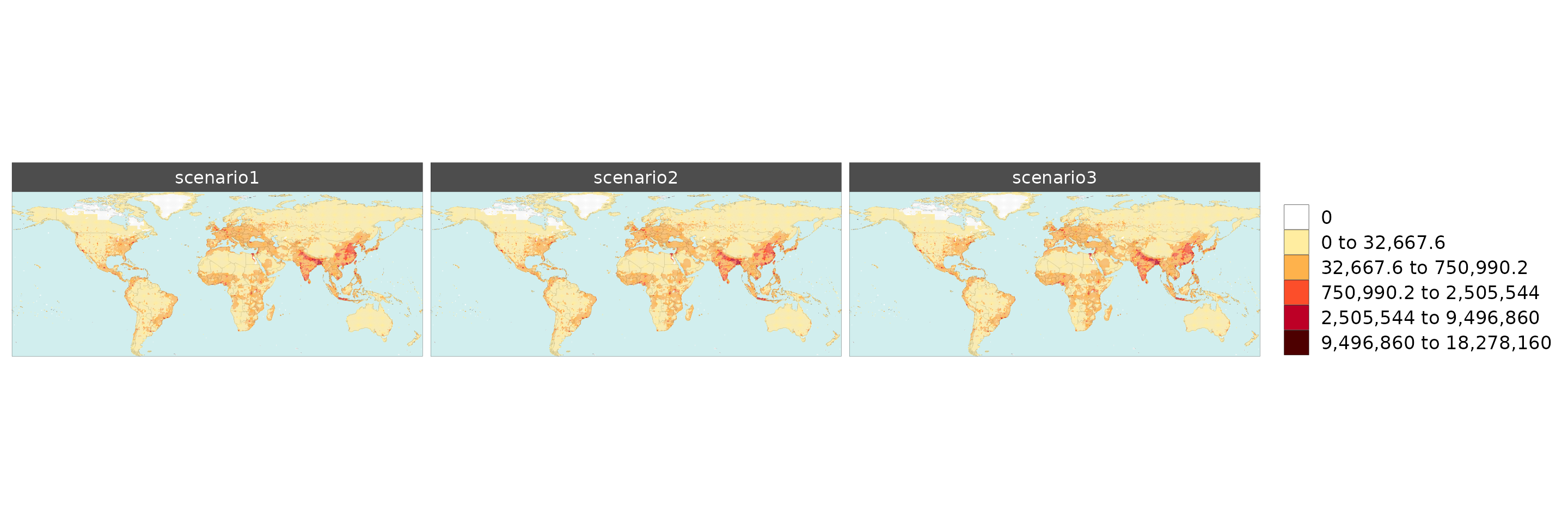
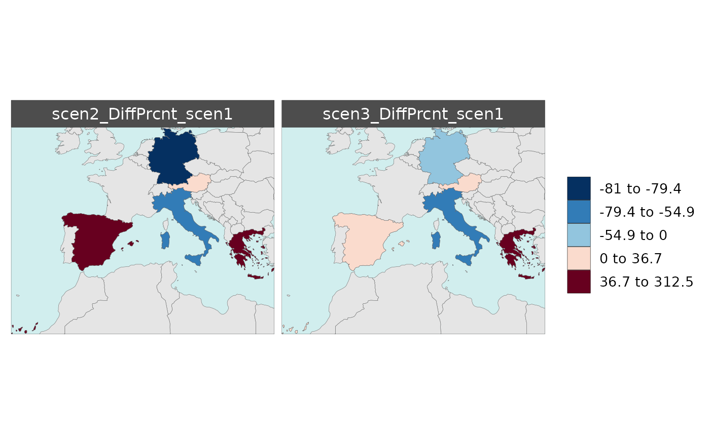
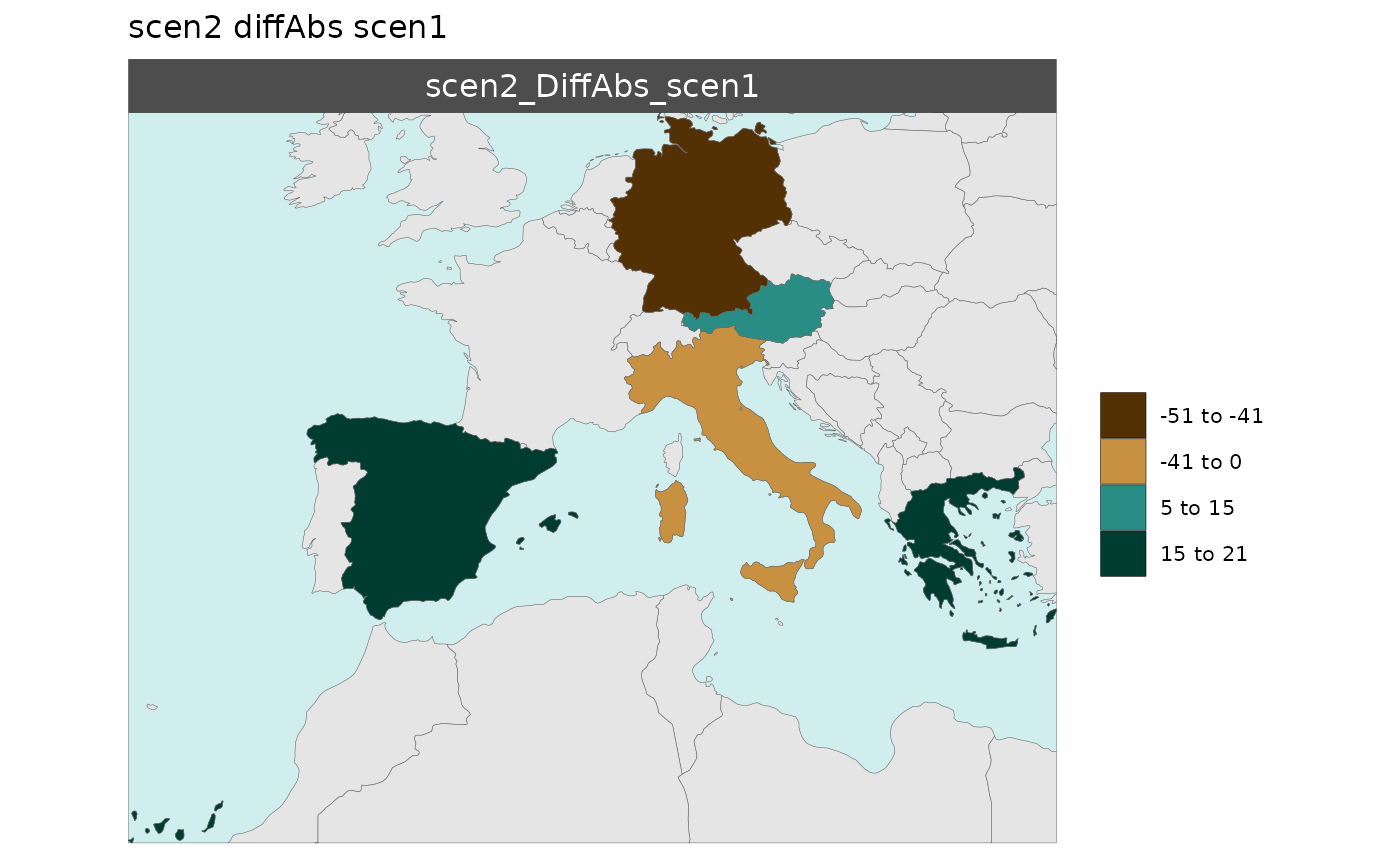
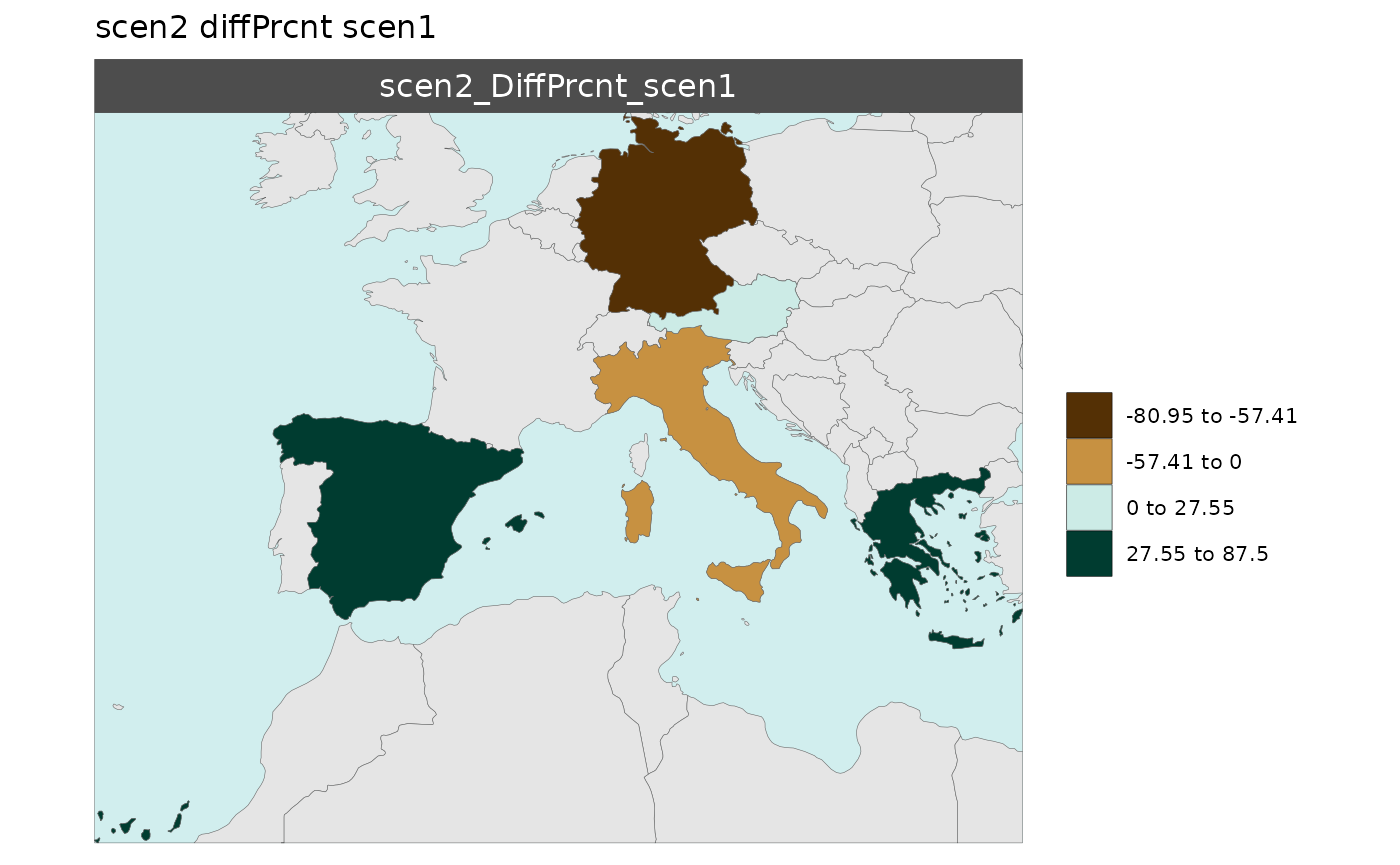
Multi-Scenario Diff Plots
With multiple scenarios present if scenRef and
scenDiff are chosen rmap::map() will produce
corresponding absolute and difference maps as shown below.
Polygon Data Multi-Scenario Diff
library(rmap);

data = data.frame(subRegion = c("Austria","Spain", "Italy", "Germany","Greece",
                                "Austria","Spain", "Italy", "Germany","Greece",
                                "Austria","Spain", "Italy", "Germany","Greece"),
                  scenario = c("scen1","scen1","scen1","scen1","scen1",
                               "scen2","scen2","scen2","scen2","scen2",
                               "scen3","scen3","scen3","scen3","scen3"),
                  value = c(32, 38, 54, 63, 24,
                            37, 53, 23, 12, 45,
                            40, 44, 12, 30, 99))
mapx <- rmap::map(data = data,
          underLayer = rmap::mapCountries,
          scenRef = "scen1",
          scenDiff = c("scen2","scen3"), # Can omit this to get difference against all scenarios
          background = T)

mapx$map_param_KMEANS_DiffAbs
mapx$map_param_KMEANS_DiffPrcnt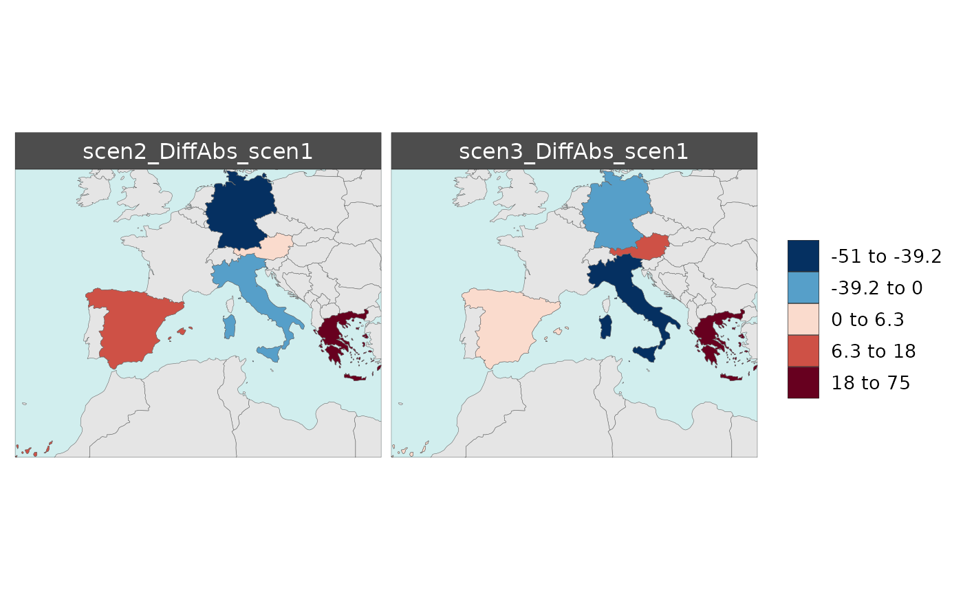
Gridded Data Multi-Scenario Diff
library(rmap); library(dplyr)

# Change the years in the example gridded data to scenarios
data = example_gridData_GWPv4To2015 %>%
  dplyr::filter(x %in% c("2000","2005","2010")) %>%
  dplyr::rename(scenario=x) %>%
  dplyr::mutate(scenario = dplyr::case_when(
    scenario == "2000" ~ "scenario1",
    scenario == "2005" ~ "scenario2",
    scenario == "2010" ~ "scenario3",
    TRUE ~ scenario))

mapx <- rmap::map(data = data,
          underLayer = rmap::mapCountries,
          scenRef = "scenario1",
          scenDiff = c("scenario2","scenario3"),
          background = T,
          ncol=1, width = 15, height =15)

mapx$map_param_KMEANS_DiffAbs
mapx$map_param_KMEANS_DiffPrcnt
Multi-Facet Maps
If the data set has additional rows and columns by which the user
wants to plot their maps they can set these in the row and
col arguments.
Polygon Data Multi-Facet
library(rmap);

data = data.frame(subRegion = c("Austria","Spain", "Italy", "Germany","Greece",
                                "Austria","Spain", "Italy", "Germany","Greece",
                                "Austria","Spain", "Italy", "Germany","Greece",
                                "Austria","Spain", "Italy", "Germany","Greece"),
                  rcp = c(rep("RCP1",5),
                          rep("RCP2",5),
                          rep("RCP1",5),
                          rep("RCP2",5)),
                  gcm = c(rep("GCM1",5),
                          rep("GCM1",5),
                          rep("GCM2",5),
                          rep("GCM2",5)),
                  value = c(32, 38, 54, 63, 24,
                            37, 53, 23, 12, 45,
                            23, 99, 102, 85, 75,
                            12, 76, 150, 64, 90))
rmap::map(data = data,
          underLayer = rmap::mapCountries,
          row = "rcp",
          col = "gcm",
          background = T )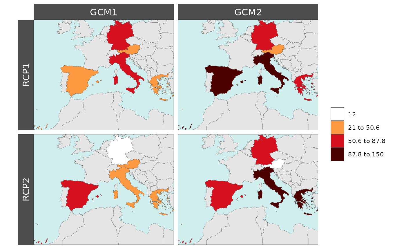
Gridded Data Multi-Facet
library(rmap);library(dplyr)

# Create data with new columns RCPs and GCMs
data = example_gridData_GWPv4To2015 %>%
  dplyr::filter(x %in% c(2000,2005,2010,2015)) %>%
  dplyr::rename(rcp = x) %>%
  dplyr::mutate(gcm = dplyr::case_when(rcp == 2000 ~ "GCM1",
                                       rcp == 2005 ~ "GCM1",
                                       rcp == 2010 ~ "GCM2",
                                       rcp == 2015 ~ "GCM2",
                                       TRUE ~ "GCM"),
                rcp = dplyr::case_when(rcp == 2000 ~ "RCP1",
                                       rcp == 2005 ~ "RCP2",
                                       rcp == 2010 ~ "RCP1",
                                       rcp == 2015 ~ "RCP2",
                                       TRUE ~ rcp))
rmap::map(data = data,
          overLayer = rmap::mapCountries,
          row= "rcp",
          col = "gcm",
          background = T,
          width=15, height =15)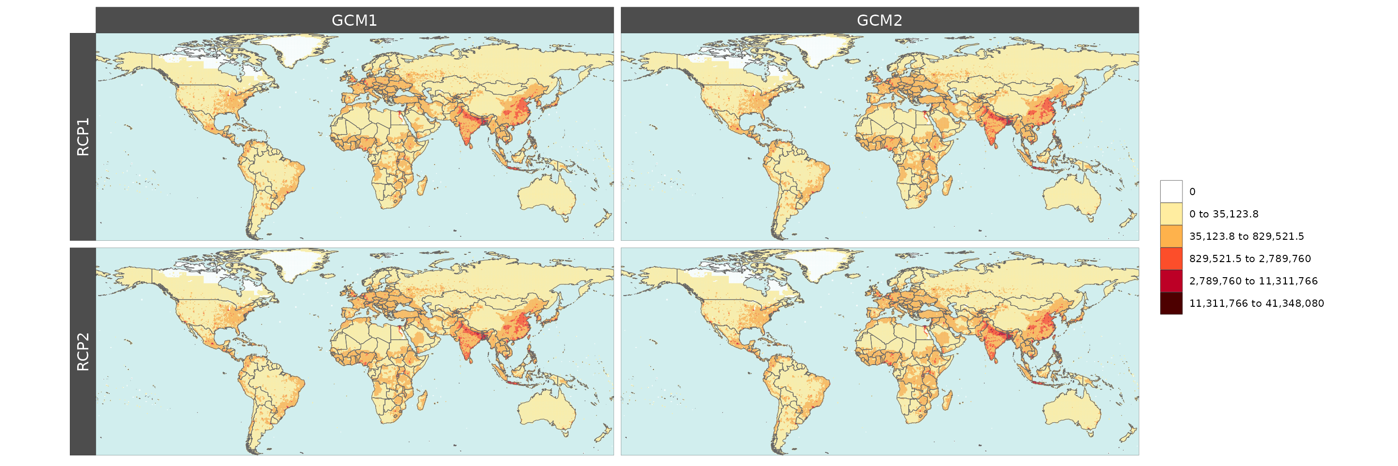
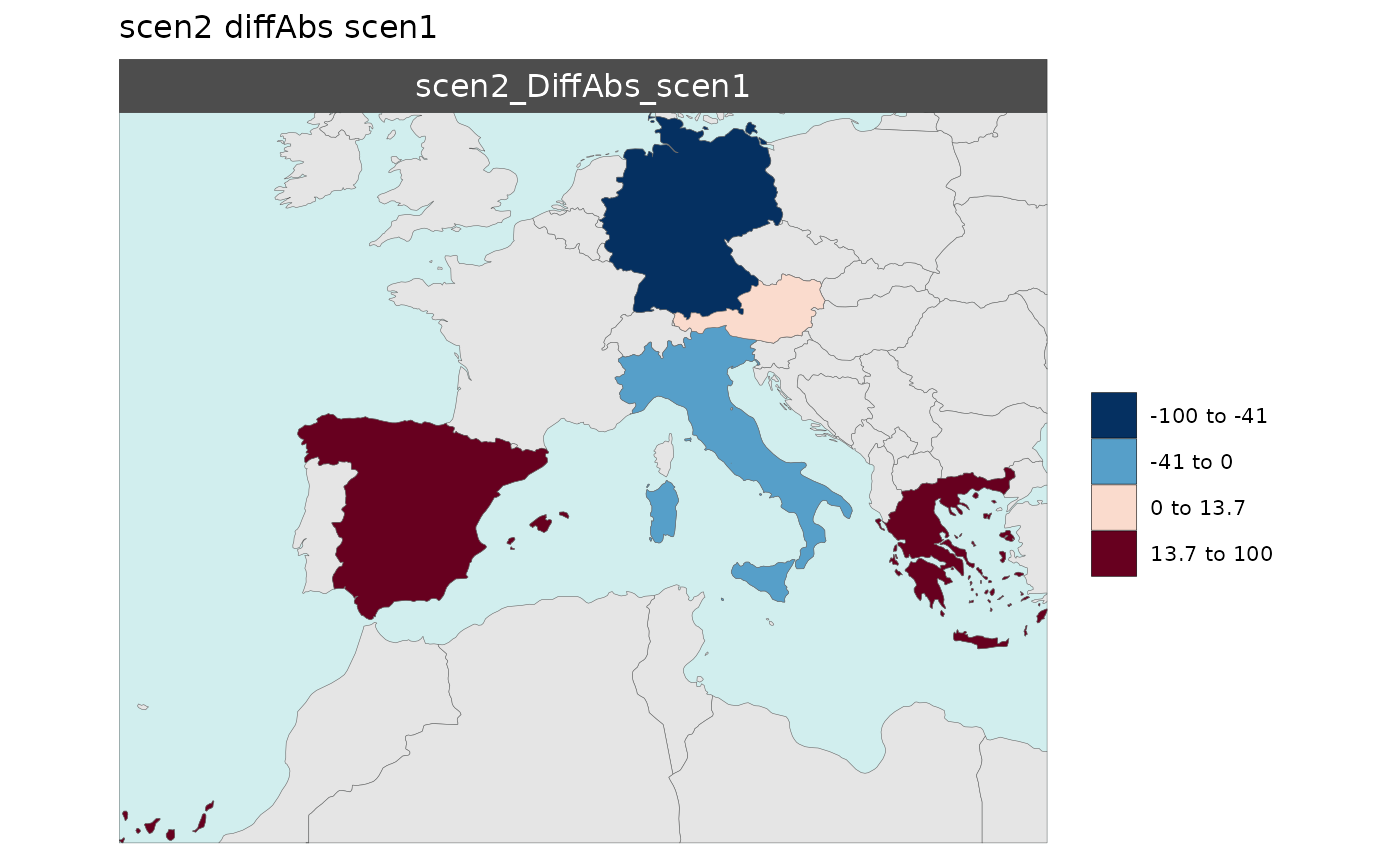
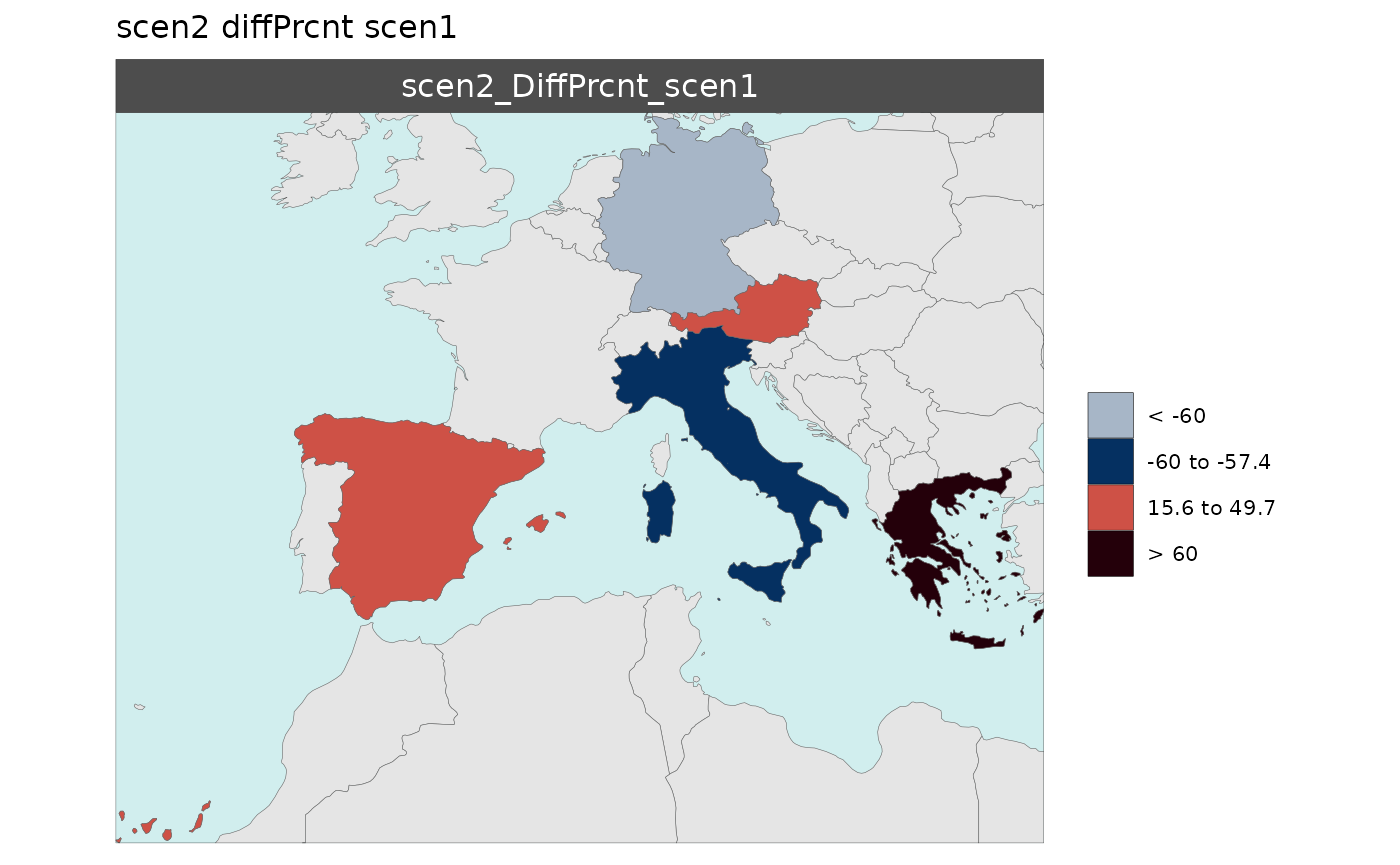
Scale Range
library(rmap)

# For Scenario Diff plots
data = data.frame(subRegion = c("Austria","Spain", "Italy", "Germany","Greece",
                                "Austria","Spain", "Italy", "Germany","Greece"),
                  scenario = c("scen1","scen1","scen1","scen1","scen1",
                               "scen2","scen2","scen2","scen2","scen2"),
                  value = c(32, 38, 54, 63, 24,
                            37, 53, 23, 12, 45))
rmap::map(data = data,
          background = T,
          underLayer = rmap::mapCountries,
          scenRef = "scen1",
          scaleRange = c(30,40),
          scaleRangeDiffAbs = c(-100,100),
          scaleRangeDiffPrcnt = c(-60,60))

# For Year Diff plots
data = data.frame(subRegion = c("Austria","Spain", "Italy", "Germany","Greece",
                                "Austria","Spain", "Italy", "Germany","Greece"),
                  x = c(rep(2010,5),
                        rep(2020,5)),
                  value = c(32, 38, 54, 63, 24,
                            37, 53, 23, 12, 45))
rmap::map(data = data,
          background = T,
          underLayer = rmap::mapCountries,
          xRef = 2010,
          forceFacets = T,
          scaleRange = c(20,30),
          scaleRangexDiffAbs = c(-70,70),
          scaleRangexDiffPrcnt = c(-150,150))

# If multiple parameters in data users can set up scaleRange for each param as:
# scaleRange_i = data.frame(param = c("param1","param2"),
#                                   min = c(0,0),
#                                   max = c(15000,2000))
# scaleRangexDiffAbs_i = data.frame(param = c("param1","param2"),
#                                   min = c(0,0),
#                                   max = c(15000,2000))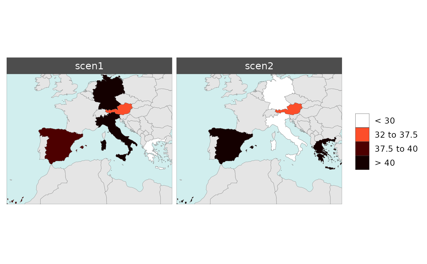
Color Palettes
Can use any R color palette or choose from a list of colors from the jgcricolors package.
library(rmap)

data = data.frame(subRegion = c("Austria","Spain", "Italy", "Germany","Greece",
                                "Austria","Spain", "Italy", "Germany","Greece"),
                  scenario = c("scen1","scen1","scen1","scen1","scen1",
                               "scen2","scen2","scen2","scen2","scen2"),
                  year = rep(2010,10),
                  value = c(32, 38, 54, 63, 24,
                            37, 53, 23, 12, 45))
rmap::map(data = data,
          underLayer = rmap::mapCountries,
          background = T,
          scenRef = "scen1",
          palette = "pal_wet",
          paletteDiff = "pal_div_BrGn")
Legend Customization
There are several options to customize your legend as shown below:
Legend Type
- There are four types of legend options (
legendType): “kmeans”, “continuous”, “pretty”, and “fixed”. - The default is “kmeans”. Users can set
legendType = "all"or any combination oflegendType = c("kmeans","pretty") - Fixed legend breaks can be set using
legendFixedBreaksto set custom and uneven breaks as shown in the example. - If
legendFixedBreaksdoes not capture the full range of data, the maximum and minimum values will be appended to the breaks provided.
Legend Fixed Breaks
library(rmap)

data = data.frame(subRegion = c("Austria","Spain", "Italy", "Germany","Greece"),
                  value = c(32, 38, 54, 63, 24))

rmap::map(data = data,
    background = T,
    underLayer = rmap::mapCountries,
    legendFixedBreaks=c(30,32,1000))  # Will append 24 to these breaks because they are part of the data.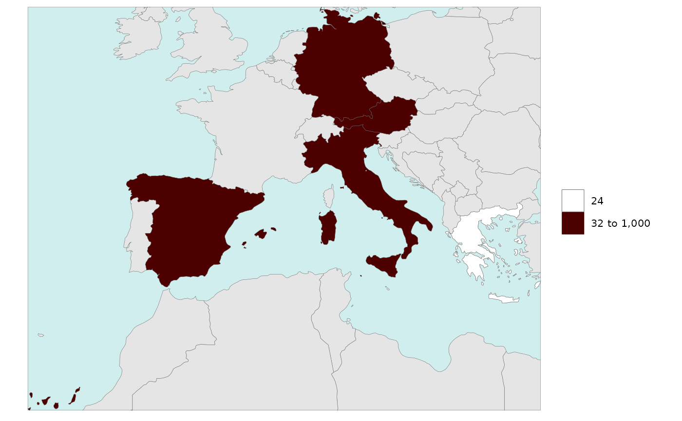
Legend Type Kmeans
library(rmap)

data = data.frame(subRegion = c("Austria","Spain", "Italy", "Germany","Greece"),
                  value = c(32, 38, 54, 63, 24))

rmap::map(data = data,
    background = T,
    underLayer = rmap::mapCountries,
    legendType = "kmeans")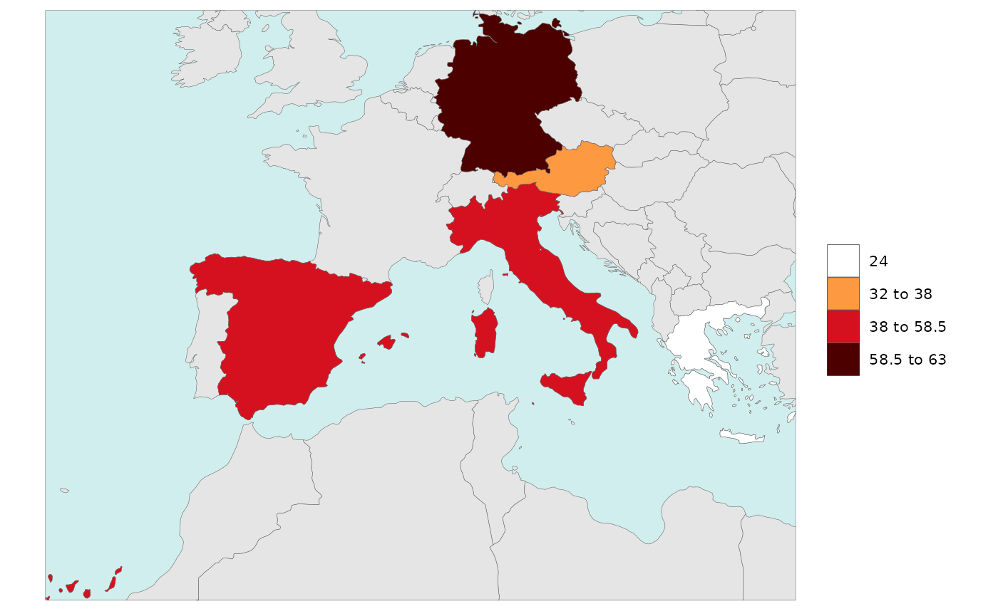
Legend Type Pretty
library(rmap)

data = data.frame(subRegion = c("Austria","Spain", "Italy", "Germany","Greece"),
                  value = c(32, 38, 54, 63, 24))

rmap::map(data = data,
    background = T,
    underLayer = rmap::mapCountries,
    legendType = "pretty")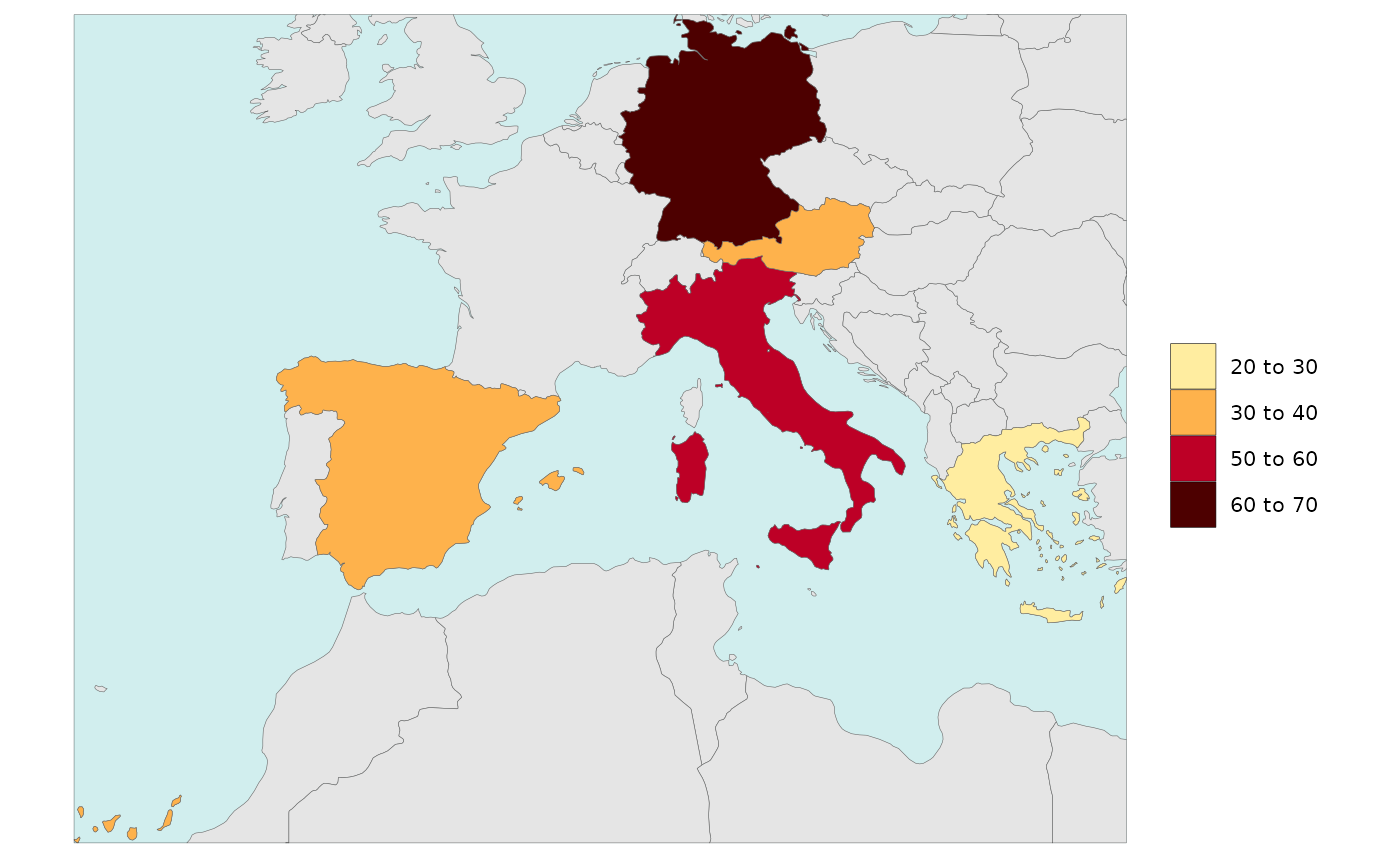
Legend Type Continuous
library(rmap)

data = data.frame(subRegion = c("Austria","Spain", "Italy", "Germany","Greece"),
                  value = c(32, 38, 54, 63, 24))

rmap::map(data = data,
    background = T,
    underLayer = rmap::mapCountries,
    legendType = "continuous")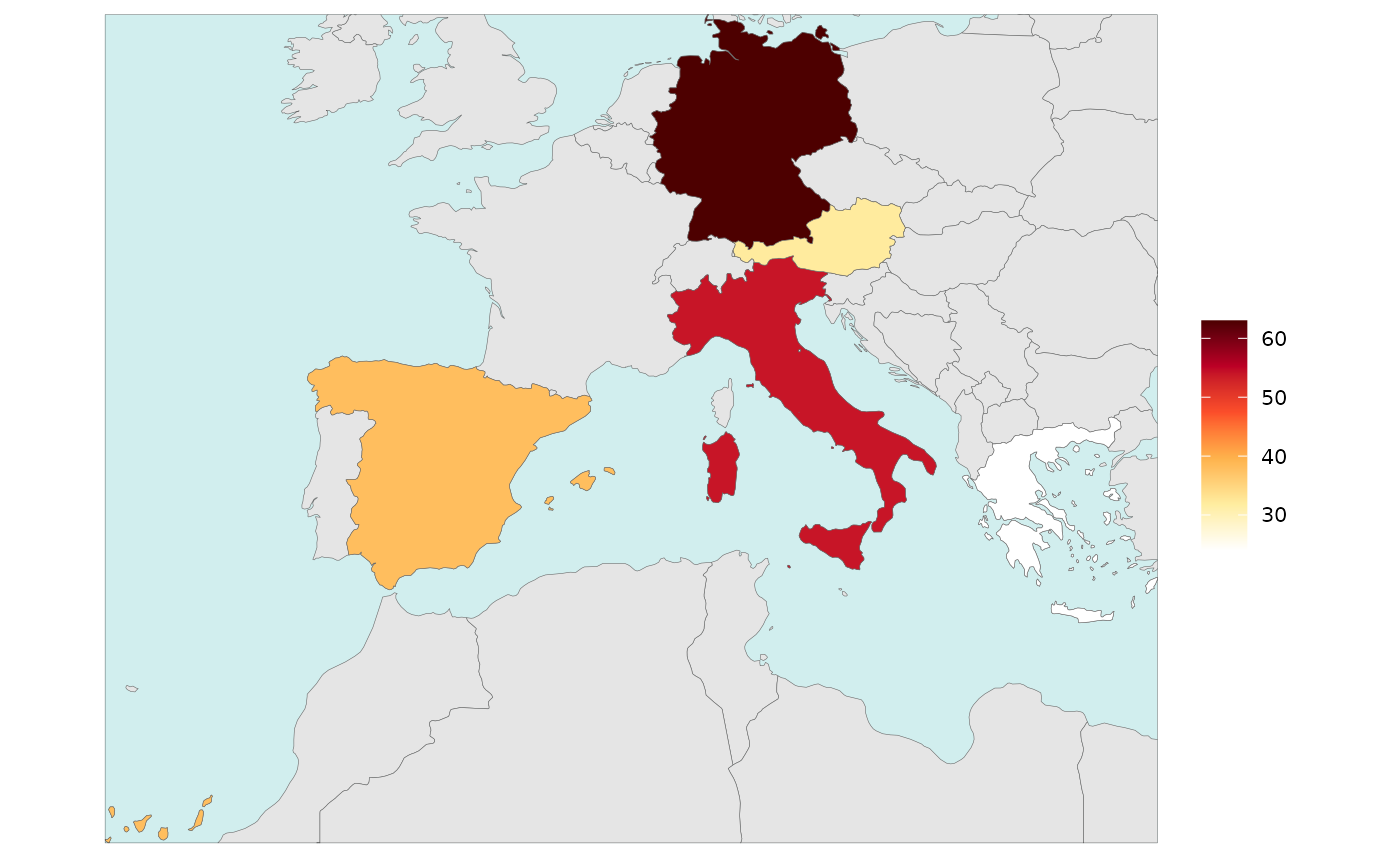
Legend Breaks Number
- Number of legend breaks can be set using the
legendBreaksnvariable. - “Pretty” legends will choose the number of breaks closest to the
value of
legendBreaksnwhile ensuring “pretty” number distributions. - “Kmeans” will ignore the value chosen for
legendBreaksnsince it calculates the best breaks it self to highlight the distribution of the data. - The
legendBreaksnwill apply in the same way to Diff Plots.
library(rmap)

data = data.frame(subRegion = c("Austria","Spain", "Italy", "Germany","Greece"),
                  value = c(32, 38, 54, 63, 24))

rmap::map(data = data,
          background = T,
          underLayer = rmap::mapCountries,
          legendType = "pretty",
          legendBreaksn=3)
rmap::map(data = data,
          background = T,
          underLayer = rmap::mapCountries,
          legendType = "pretty",
          legendBreaksn=9)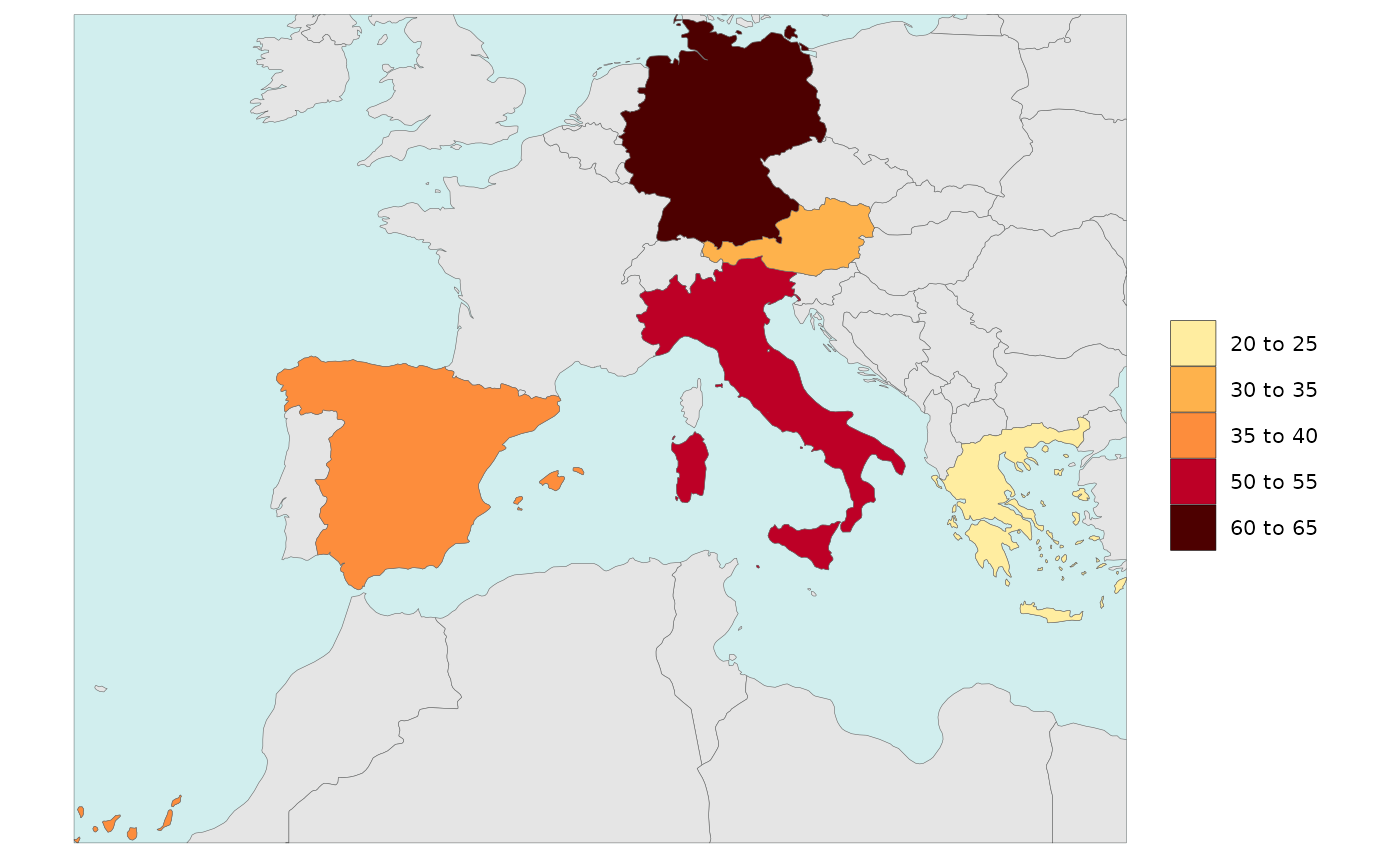
Legend Single Value
Users can add a single value to the legend ranges. Sometimes it is
important to see the 0 or minimum value in a rnage of data
and this allows users to do that. Users can simply set
legendSingleValue=T to use the minimum value (or 0 if
present) of their dataset as the minimum value or set the value to a
particular number. Users cna also set the color of the single value they
choose as shown in the examples below.
library(rmap)

data = data.frame(subRegion = c("Austria","Spain", "Italy", "Germany","Greece"),
                  value = c(-5,0, 54, 63, 24))

# Without single value turned on
rmap::map(data = data,
          background = T,
          underLayer = rmap::mapCountries)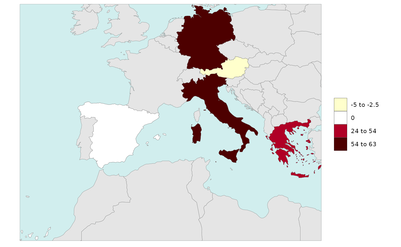
# With legendSingelValue = T (will choose the minimum value or if 0 (if present) and set it to single)
rmap::map(data = data,
          background = T,
          underLayer = rmap::mapCountries,
          legendSingleValue = T)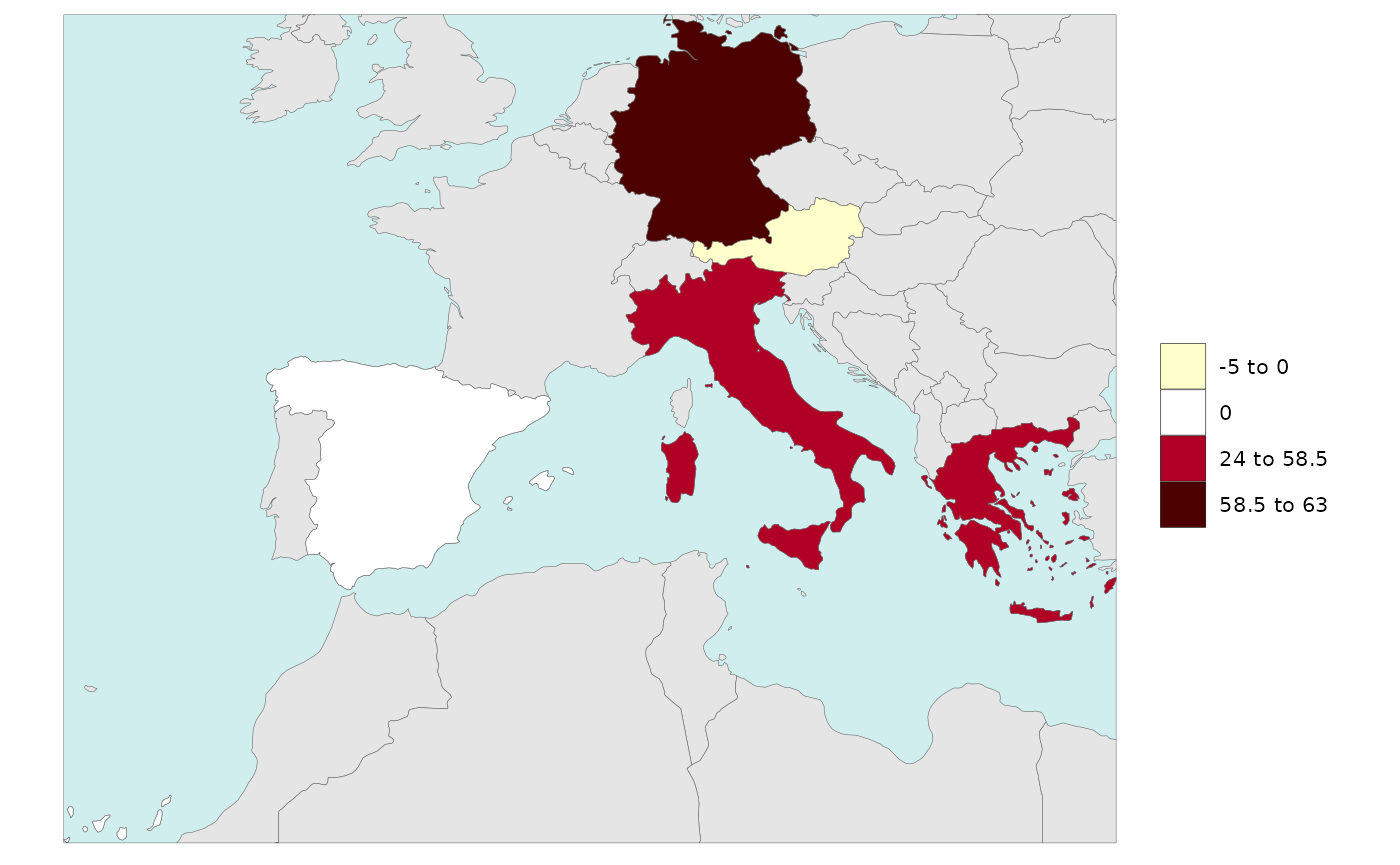
# With legendSingelValue = 38 and set to "green"
rmap::map(data = data,
          background = T,
          underLayer = rmap::mapCountries,
          legendSingleValue = 54,
          legendSingleColor = "green")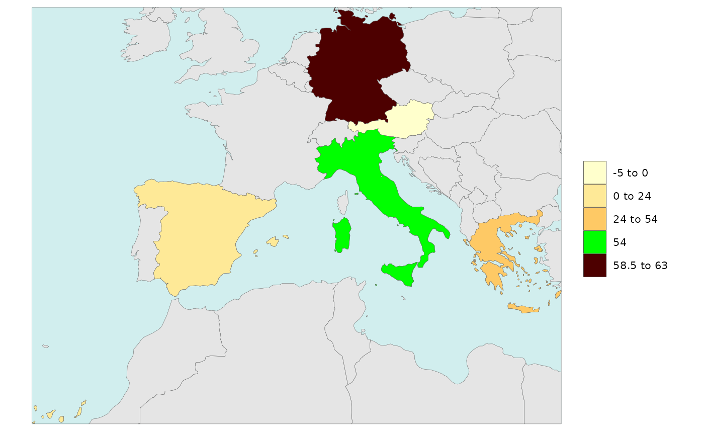
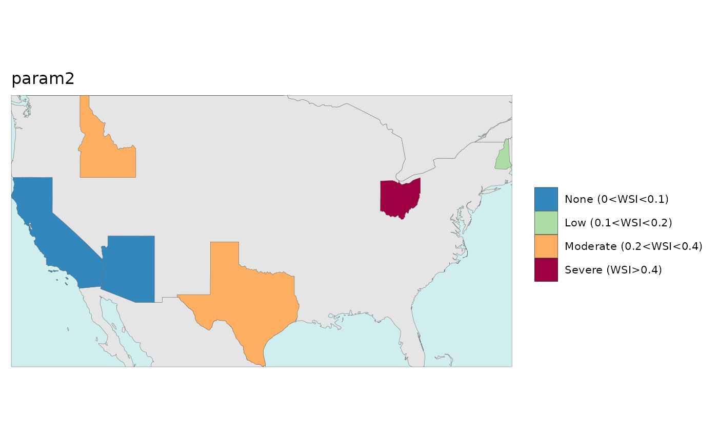
Numeric2Cat
The numeric2cat parameter in the map function allows
users to assign their own categorical legend labels for chosen ranges of
numeric values.
library(rmap);library(jgcricolors)

# Create a list of ranges and categorical color scales for each parameter
numeric2Cat_param <- list("param1",
                          "param2")
numeric2Cat_breaks <- list(c(-Inf, 0.1,1.1,2.1,3.1,4.1,5.1,10.1,Inf),
                           c(-Inf, 0.1, 0.2, 0.4,Inf))
numeric2Cat_labels <- list(c("0","1","2","3","4","5","10",">10"),
                           c(names(jgcricolors::jgcricol()$pal_scarcityCat)))
numeric2Cat_palette <- list(c("0"="green","1"="#fee5d9","2"="#fcbba1",
                              "3"="#fc9272","4"="#fb6a4a","5"="#de2d26",
                              "10"="#a50f15",">10"="black"),
                            c("pal_scarcityCat")) # Can be a custom scale or an R brewer palette or an rmap palette
numeric2Cat_legendTextSize <- list(c(0.7),
                                   c(0.7))
numeric2Cat_list <-list(numeric2Cat_param = numeric2Cat_param,
                        numeric2Cat_breaks = numeric2Cat_breaks,
                        numeric2Cat_labels = numeric2Cat_labels,
                        numeric2Cat_palette = numeric2Cat_palette,
                        numeric2Cat_legendTextSize = numeric2Cat_legendTextSize); numeric2Cat_list

data = data.frame(subRegion = c("CA","AZ","TX","NH","ID","OH",
                              "CA","AZ","TX","NH","ID","OH"),
                  x = c(2050,2050,2050,2050,2050,2050,
                      2050,2050,2050,2050,2050,2050),
                  value = c(0,1,3,20,2,1,
                          0,0.1,0.3,0.2,0.25,0.5),
                  param = c(rep("param1",6),rep("param2",6)))

rmap::map(data = data,
          background = T,
          underLayer = rmap::mapCountries,
          numeric2Cat_list = numeric2Cat_list)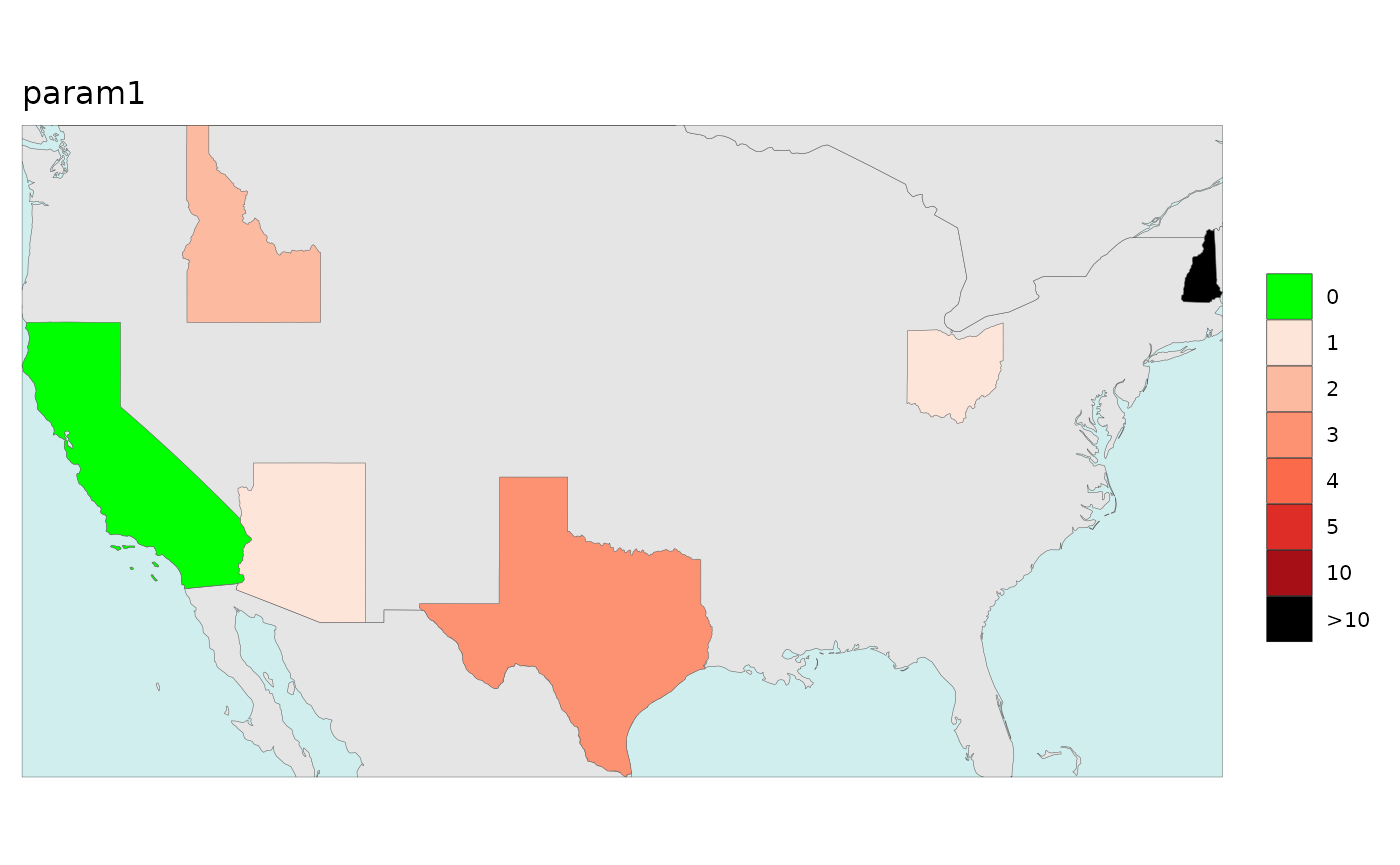
GCAM Results & Examples
GCAM Basins
GCAM Basins can come sometimes come abbreviated. To covnert these
into the names associated with the rmap::mapGCAMBasin basin
names the following mapping is provided:
rmap::mapping_gcambasins # View the mapping
# Convert
data <- data %>%
dplyr::left_join(rmap::mapping_gcambasins,by="subRegion")%>%
dplyr::mutate(subRegion=dplyr::case_when(!is.na(subRegionMap)~subRegionMap,
TRUE~subRegion))%>%
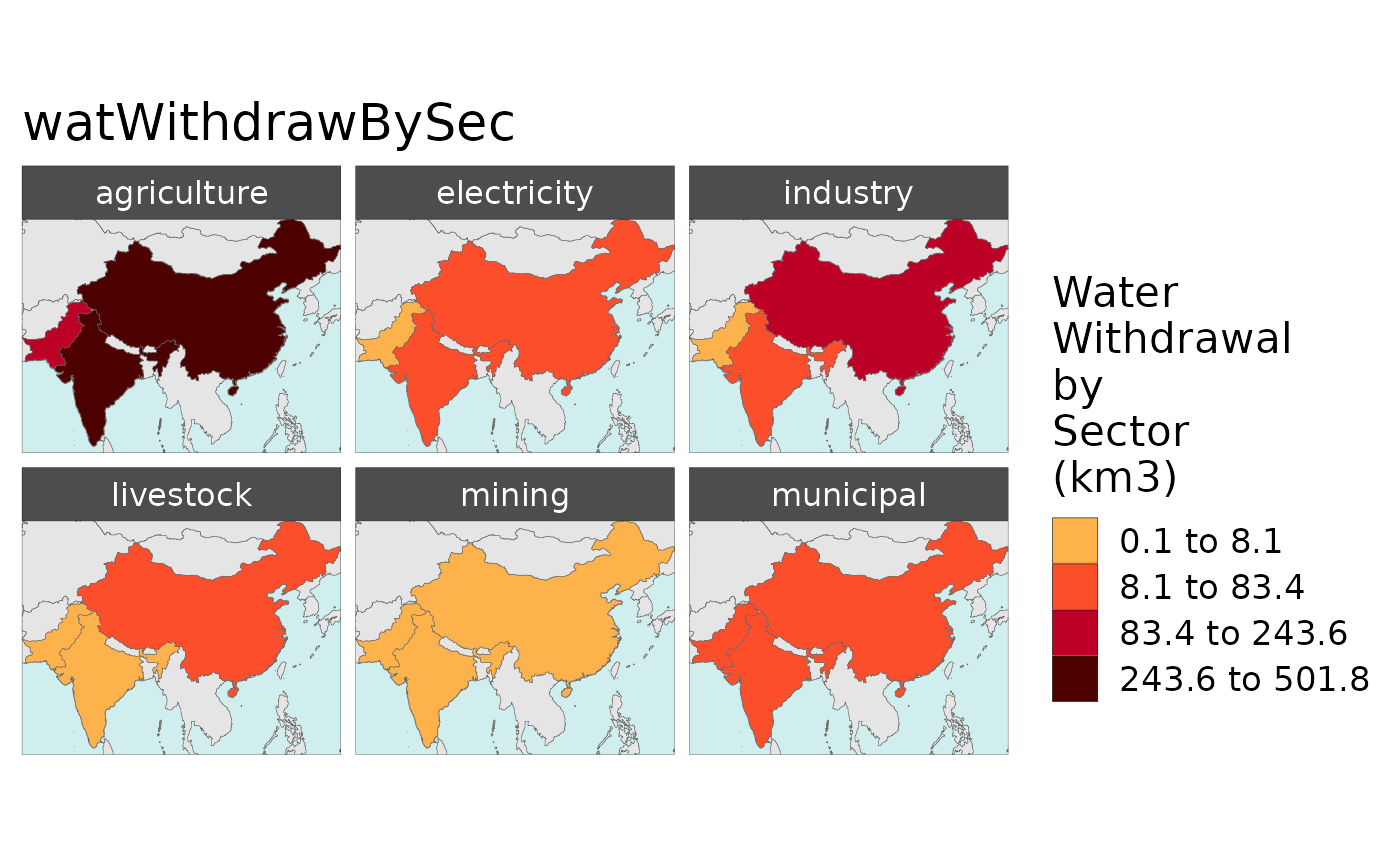
dplyr::select(-subRegionMap)GCAM Param Example
In this example data was extracted from a GCAM output database and
aggregated by paramater and class into
rmap::exampleMapDataParam and
rmap::exampleMapDataClass. Users can process their own GCAM
data outputs into similar tables using the gcamextractor R
package available at https://jgcri.github.io/gcamextractor/.
Note: The example data comes with only a few parameters: “elecByTechTWh”,“pop”,“watWithdrawBySec”,“watSupRunoffBasin”,“landAlloc” and “agProdByCrop”
library(rmap)

dfClass <- rmap::exampleMapDataClass %>%
  dplyr::filter(region %in% c("India","China","Pakistan"),
                param %in% c("watWithdrawBySec"),
                x %in% c(2010),
                scenario %in% c("GCAM_SSP3")); dfClass


# Plot data aggregated by Class1
rmap::map(data = dfClass,
          background = T,
          underLayer = rmap::mapGCAMReg32,
          save=F)