Structure

plutus::gcamInvest integrates the functionality of reading CGAM database and calculating stranded assets and electricity investments in the power sector. This function will return a list containing:
- data: a dataframe with the post-processed GCAM output showing stranded assets and electricity investment (see Table 1) by scenario, region, technology, and time period
- dataAggParam: a dataframe with the data aggregated to the parameter
- dataAggClass1: a dataframe with the data aggregated to class 1
- dataAggclass2: a dataframe with the data aggregated to class 2
- scenarios: A list of the scenarios
- queries: A list of the queries used to extract the data
Table 1: Descriptions of output parameters for stranded assets and electricity investments.
| Parameter | Description | Unit |
|---|---|---|
| elecNewCapCost | 5-year electricity capacity installations | Billion 2010 USD |
| elecNewCapGW | 5-year electricity capacity installations | Gigawatts |
| elecAnnualRetPrematureCost | 5-year premature retirements | Billion 2010 USD |
| elecAnnualRetPrematureGW | 5-year premature retirements | Gigawatts |
| elecCumCapCost | Cumulative electricity capacity installations | Billion 2010 USD |
| elecCumCapGW | Cumulative electricity capacity installations | Gigawatts |
| elecCumRetPrematureCost | Cumulative premature retirements | Billion 2010 USD |
| elecCumRetPrematureGW | Cumulative premature retirements | Gigawatts |
The details of arguments and their default values in plutus::gcamInvest can be found in the gcamInvest reference page. The following sections provide step-by-step instructions on using plutus::gcamInvest.
# Default argument values
plutus::gcamInvest(gcamdatabase = NULL,
                   queryFile = NULL,
                   reReadData = T,
                   dataProjFile = paste(getwd(), "/outputs/dataProj.proj", sep = ""),
                   gcamdataFile = NULL,
                   scenOrigNames = 'All',
                   scenNewNames = NULL,
                   regionsSelect = NULL,
                   dirOutputs = paste(getwd(), "/outputs", sep = ""),
                   folderName = NULL,
                   nameAppend = "",
                   saveData = T)
Read GCAM Data
Read .proj File
plutus::gcamInvest is able to read rgcam-based .proj file from GCAM output by providing the path to the .proj file. plutus also includes an example .proj dataset plutus::exampleGCAMproj.
library(plutus)

invest <- plutus::gcamInvest(# dataProjFile = path_to_projfile,
                             dataProjFile = plutus::exampleGCAMproj)

# Explore the list returned from plutus::gcamInvest
df <- invest$data; df
dfParam <- invest$dataAggParam; dfParam
dfClass1 <- invest$dataAggClass1; dfClass1
dfScenario <- invest$scenarios; dfScenario
dfQuery <- invest$queries; dfQuery
Read GCAM XML Database
plutus::gcamInvest can directly read GCAM output XML database. Assign the path of GCAM database to gcamdatabase argument.
library(plutus)

# provide path to the desired GCAM database folder.
path_to_gcamdatabase <- 'E:/gcam-core-gcam-v5.3/output/databse_basexdb'
invest <- plutus::gcamInvest(gcamdatabase = path_to_gcamdatabase)
Subset GCAM Data
plutus::gcamInvest provides options to subset GCAM data by scenario and region.
library(plutus)

invest <- plutus::gcamInvest(dataProjFile = plutus::exampleGCAMproj,
                             scenOrigNames = c('Reference', 'Impacts', 'Policy'),
                             scenNewNames = c('Reference', 'Climate Impacts', 'Climate Policy'),
                             regionsSelect = c('USA', 'Argentina'))

df <- invest$data; df
dfParam <- invest$dataAggParam; dfParam
dfClass1 <- invest$dataAggClass1; dfClass1
Input Data and Assumptions
plutus provides default data and assumptions files from GCAM v5.3 that are collected from Default-GCAM-5.3-Folder/input/gcamdata/. All data files (CSV) associated with different data categories and assumptions are listed in Table 2.
Table 2: Data and assumption files.
| Data or Assumption | Technology | Region | Data File |
|---|---|---|---|
| Overnight capital costs | Electricity generation technologies | Global | L2233.GlobalIntTechCapital_elec.csv L2233.GlobalTechCapital_elecPassthru.csv |
| Overnight capital costs | Cooling technologies | Global | L2233.GlobalIntTechCapital_elec_cool.csv L2233.GlobalTechCapital_elec_cool.csv |
| Capacity factors | Electricity generation technologies | Global | L223.GlobalTechCapFac_elec.csv |
| Capacity factors | Intermittant technologies | Global | L223.GlobalIntTechCapFac_elec.csv |
| Capacity factors | Intermittant technologies | Regional | L223.StubTechCapFactor_elec.csv |
| Lifetime and steepness | Electricity generation technologies | Global | A23.globaltech_retirement.csv |
However, users may run GCAM v5.3 with updated/customized values associated with capital costs, capacity factors, and lifetime by technology and region. In this case, plutus::gcamInvest allows users to input their own data associated with their GCAM runs. All you need to do is to provide the path that includes ALL CSV files listed in Table 2. Here are two options:
- Users can update CSV files listed in Table 2 directly in Your-GCAM-5.3-Folder/input/gcamdata. Then, specify argument to
gcamdataFile = Your-GCAM-5.3-Folder/input/gcamdata. - Users can copy and paste all CSV files listed in Table 2 from Your-GCAM-5.3-Folder/input/gcamdata to a new folder and update the values according to your GCAM run. Then, specify argument to
gcamdataFile = Path-to-Your-New-Folder.
While updating the values in those CSV files, please keep the file name and the format of each updated file unchanged.
library(plutus)

invest <- plutus::gcamInvest(dataProjFile = plutus::exampleGCAMproj,
                             gcamdataFile = 'E:/gcam-core-gcam-v5.3/input/gcamdata')
Output Options
plutus::gcamInvest automatically saves outputs, such as .proj files, queries, and output data tables in default path based on the working directory. This section will introduce arguments in plutus::gcamInvest that control different output options.
Re-read Data
plutus::gcamInvest automatically save a copy of .proj file (default name: dataProj.proj) in the output directory after extracting GCAM output data if provided a GCAM database folder using gcamdatabase argument. Reload the same (subsetted) GCAM dataset can be much faster by using the automatically saved dataProj.proj file. Users can choose to turnoff auto save function by specifying argument to reReadData = F.
library(plutus)

path_to_gcamdatabase <- 'E:/gcam-core-gcam-v5.3/output/databse_basexdb'
invest <- plutus::gcamInvest(gcamdatabase = path_to_gcamdatabase,
                             reReadData = F) # Default is reReadData = T
Output Directory
It is easy to change output folder names and names appended to the output data tables.
-
folderNamecreates a folder with the specified name under output directory -
nameAppendappends the specified string at the end of each output data table file
library(plutus)

invest <- plutus::gcamInvest(dataProjFile = plutus::exampleGCAMproj,
                             # dirOutputs = Your-desired-output-path, # Default is paste(getwd(), "/outputs", sep = "")
                             folderName = 'USA', # Default is fodlerName = NULL
                             nameAppend = '_Invest') # Default is nameAppend = ''
You can also choose not to save any output by setting argument to saveData = F.
library(plutus)

invest <- plutus::gcamInvest(dataProjFile = plutus::exampleGCAMproj,
                             saveData = F) # Default is saveData = T
Visualization
plutus is designed to integrate with metis (Khan et al., 2020), an R package to harmonize and analyze multi-sectoral data and linkages at variable spatial scales. plutus::gcamInvest generates a data structure that can be directly used by metis. More details on metis can be accessed via metis repository at https://github.com/JGCRI/metis.
Charts
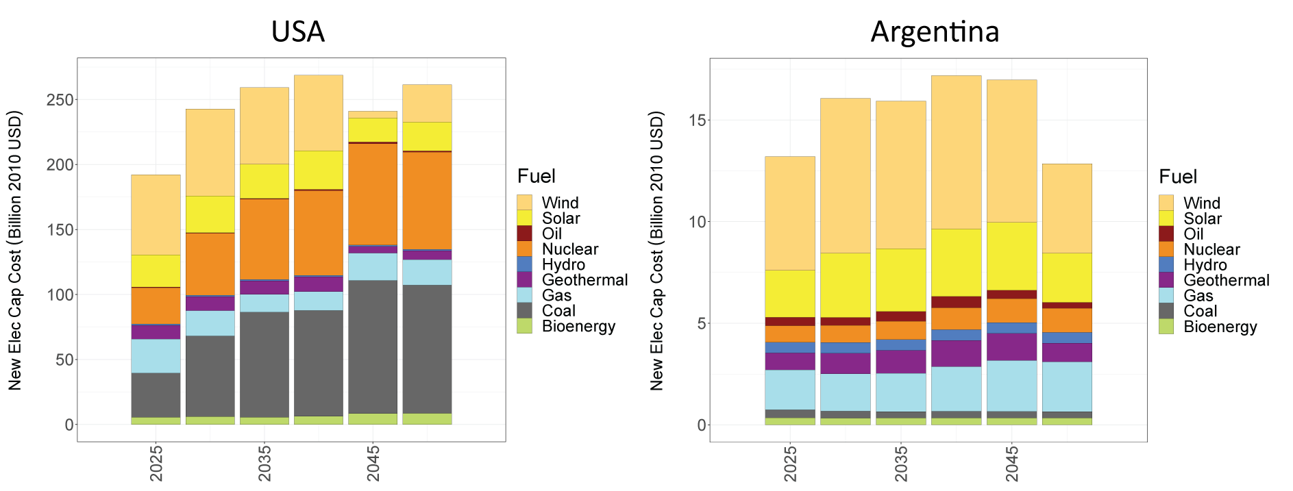
Below is an example of using metis.chartsProcess to generate charts of stranded assets and electricity investments in the USA and Argentina.
library(plutus)
library(metis)

invest <- plutus::gcamInvest(dataProjFile = plutus::exampleGCAMproj,
                             scenOrigNames = c('Reference', 'Impacts', 'Policy'),
                             scenNewNames = c('Reference', 'Climate Impacts', 'Climate Policy'),
                             regionsSelect = c('USA', 'Argentina'))
rTable_i <- invest$data

# Plot charts for each scenario and comparison between scenarios and regions across time series
metis.chartsProcess(rTable = rTable_i,
                    paramsSelect = 'All',
                    regionsSelect = c('USA', 'Argentina'),
                    xCompare = c("2030", "2040", "2050"),
                    scenRef = "Reference",
                    dirOutputs = paste(getwd(), "/outputs", sep = ""),
                    regionCompare = 1,
                    scenarioCompareOnly = 1,
                    multiPlotOn = T,
                    multiPlotFigsOnly = T,
                    folderName = "Charts_USA_Argentina",
                    xRange = c(2025, 2030, 2035, 2040, 2045, 2050),
                    colOrderName1 = "scenario",
                    pdfpng = 'pdf')
New Electricity Capacity Installations for USA and Argentina
Maps
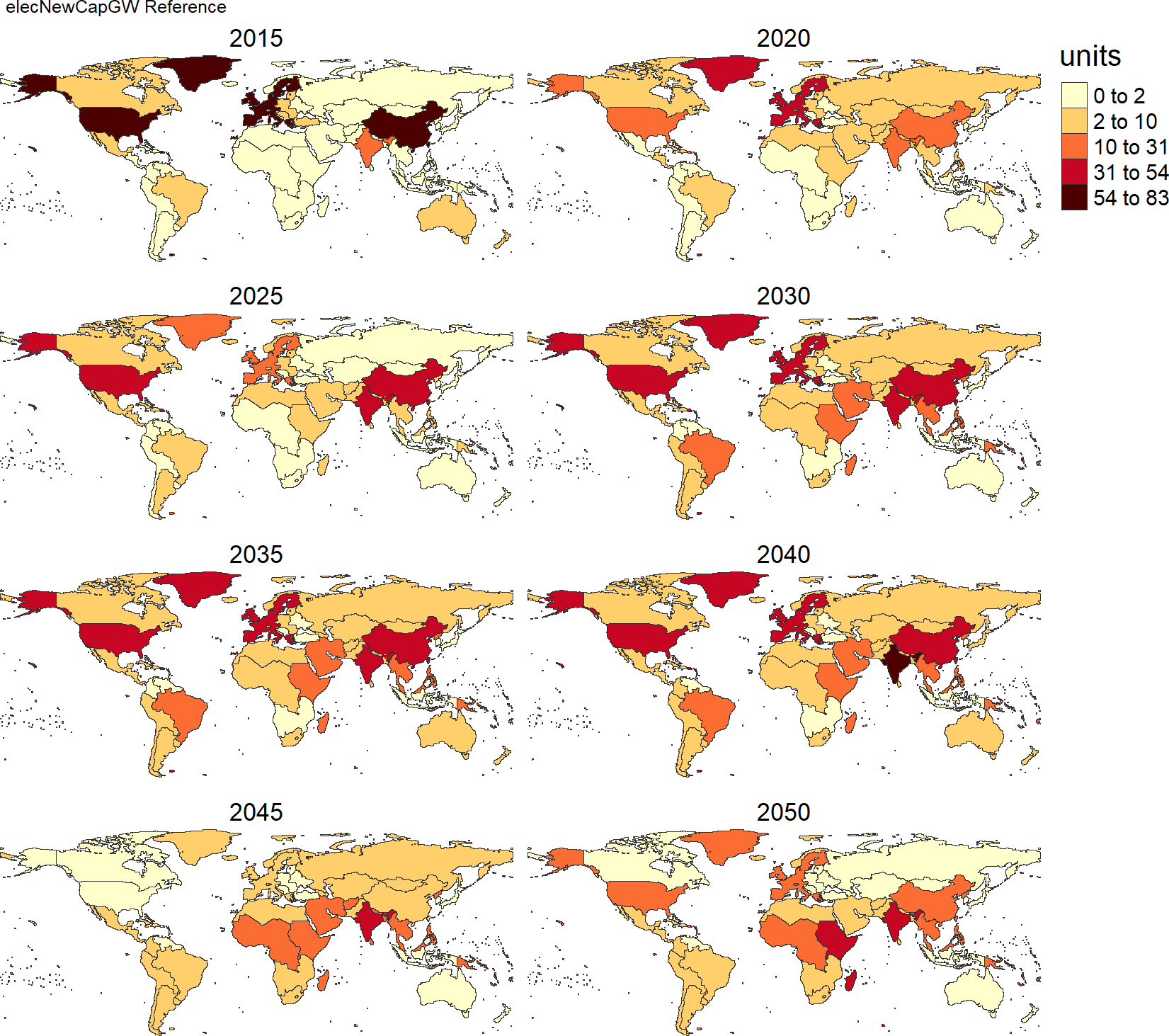
Users can also use metis.mapsProcess to produce spatial maps by scenario, region, technology, and time period. Here is an example to map wind capacity installations for 32 geopolitical regions.
library(plutus)
library(metis)

invest <- plutus::gcamInvest(dataProjFile = plutus::exampleGCAMproj,
                             scenOrigNames = 'Reference',
                             regionsSelect = NULL,
                             saveData = F)

rTable_i <- invest$data
# Filter data to only show new installations for wind
polygonTable_i <- rTable_i %>%
  dplyr::filter(class1 %in% 'Wind', param %in% 'elecNewCapGW') %>%
  dplyr::select(subRegion, value, x, class1, scenario, param) %>%
  dplyr::rename(class = class1)

# Plot wind new installation maps for all 32 geopolitical regions across time
metis.mapsProcess(polygonTable = polygonTable_i,
                  subRegCol = 'subRegion',
                  subRegType = 'subRegion',
                  folderName = 'Maps_Wind_eleNewCapGW',
                  facetCols = 2,
                  animateOn = F)
Regional Electricity Capacity Installations for Wind Technology