3. Analysis

Querying a large ensemble of GCAM outputs will most likely be done on the computing cluster which stores the databases. R will need to be installed in order to use rgcam, an R package that extracts GCAM database output into readable data formats. In a standard GCAM installation, main queries can be found in gcam-core/output/queries/Main_queries.xml and can also be customized to fit specific needs. It can be helpful to query a single model realization to see the resulting size of the output csv. Many queries can be aggregated at different levels, and individual regions, basins, model years, etc., can be specified.

Scenario discovery relies on machine learning and other statistical methods to reveal patterns in many-dimensional data. Clusters of realizations with shared input conditions leading to similar outcomes, tradeoffs, synergies, and temporal dynamics are termed “scenarios’’, which are generally framed to be interpretable, scientific or strategy-relevant insights. Note that GCAM terms each model run a “scenario”, but for the purposes of scenario discovery and other RDM tools, a more appropriate terminology would be “realization”, “simulation”, “model run”, or “ensemble member”, not to be used interchangeably with “scenario” to avoid confusion or ambiguity.

There are many algorithms capable of describing the similarity or difference between data. A common class of techniques used in scenario discovery is ensemble trees, an extension of Classification and Regression Trees (CART), as they produce interpretable and intuitive analyses and can handle nonlinear data. Additionally, other clustering algorithms such as k-means, k-medoids, and time series clustering can be used to generate scenario typologies, while dimensionality reduction techniques like PCA can also quantify important drivers of outcomes. Other feature importance or feature selection methods commonly used include Shapley values as well as various regression techniques like logistic regression, ridge, and lasso.

Ensemble tree methods include variations such as bootstrap aggregation (bagging), boosted decision trees, and random forests. Classification can be used to determine outcomes beyond a specified threshold or in an extreme region of the output space, while regression can reveal more general drivers of outcomes. The “predictors” or “features” used to train such models are the sensitivities varied in the ensemble, while the response variables are the chosen metrics. When using these models for prediction, the data should be split into training, validation, and test sets. In addition to producing decision tree figures, quantifying the influence of each predictor can be done using a feature importance analysis, which broadly determines the impact that the inclusion of each predictor has on the model performance. This can be measured as a reduction in MSE, an improvement in the Gini index, etc., and can generally be performed with statistical software packages such as scikit-learn or statsmodels for Python, and rpart or randomForest for R. Note that the feature importance will change depending on the subset of the data used. Therefore, feature importances can be computed across regions, basins, timesteps, etc. Additionally, ensemble tree methods will give scores for each tree generated, allowing for uncertainty in the feature importance to be reported. Feature importance algorithms in general may be based on different underlying statistical assumptions (which can affect how a score is interpreted) and perform differently depending on the data types of input features (causing differences in feature importance scores and rankings across techniques), so the choice of methods should consider the suite of available tools.

Computing the variability of the effect each driver has on the metrics of interest can be done by taking the difference in outcomes between pairs of realizations which differ only by a single sensitivity. Doing so across the scenario ensemble will produce a distribution, which can be shown using boxplots, CDFs, or one-to-one scatterplots. In addition to showing the magnitude of each driver’s influence, interactive effects can be computed using a variance decomposition such as Sobol sensitivity analysis, available via SALib in Python. Further, partial dependence plots can show a model’s sensitivity to a given feature across its input space.

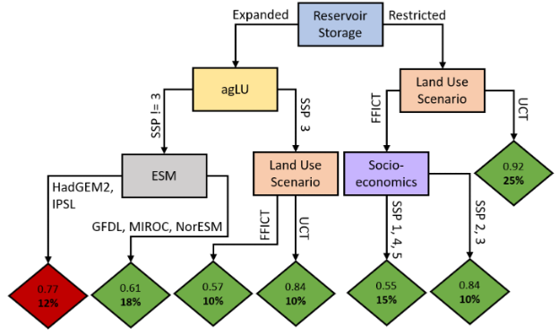
Fig. 3.1 Courtesty of Dolan et al. [3]: CART classification of positive versus negative economic impact summed over time in the Orinoco Basin. Red end nodes represent negative impact subgroups and green end nodes represent positive impact subgroups. The fraction at the top of each node shows the purity of each node, while the percentage in each end node is the percent of total scenarios within that subgroup.