GCAM v8.2 Documentation: Additional details about the energy model
Documentation for GCAM
The Global Change Analysis Model
View the Project on GitHub JGCRI/gcam-doc
Additional details about the energy model
This page provides more detailed explanations of the descriptions provided in the Energy Supply and Energy Demand modeling pages.
Table of Contents
Resources
Depletable Resources
The figures below show some illustrative examples of supply curves used within GCAM.
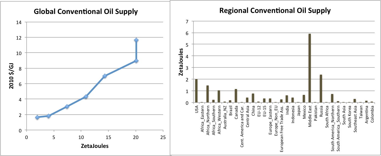
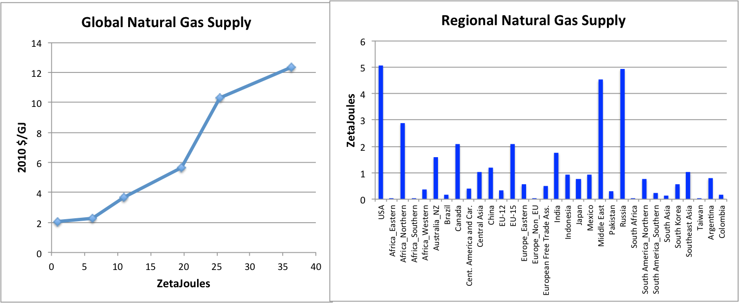
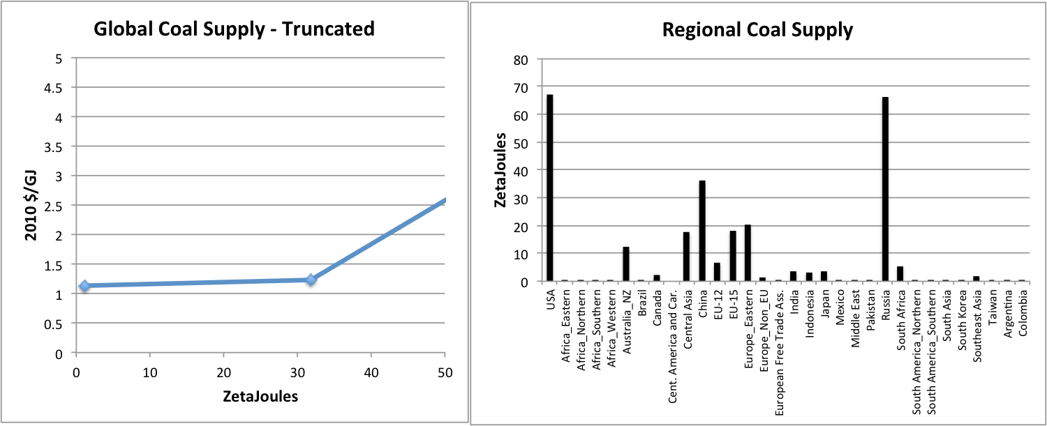
Illustrative examples of supply curves and total supplies for fossil resources in GCAM
Representation of unconventional oil as a technology within crude oil
Unconventional oil and crude oil are represented as distinct subresources within a single resource (crude oil). Combining these oil types into a one resource allows for a single price that governs supply expansion. The additional costs and energy inputs related to unconventional oil production are represented in the technology contained within the unconventional oil subresource.
Renewable Resources
Wind
The supply curves in each region are derived from bottom-up analysis documented in Eurek et al. (2017).
Solar
Distributed PV capacity factors are scaled across GCAM regions by the average latitude tilt irradiance for that region. The average latitude tilt irradiance for each country is derived from the “Latitude Tilt Radiation” variable from the NASA Surface meteorology and Solar Energy (SSE) Release 6.0 Data Set and averaged for each GCAM region. Forest and cropland areas are excluded.
The “distributed_PV” supply curve is of the same functional form as the wind supply curve, with an upward-sloping function designed to capture the increases in costs with deployment. In the USA region, the distributed_PV supply curve is estimated from data compiled by Denholm (2008). The curve-exponent is assumed the same in all other regions, the mid-prices are adjusted according to the irradiance in each region, and the maxSubResources are adjusted according to the estimated building floorspace.
Concentrated Solar Power (CSP) capacity factors across GCAM regions depend on Direct Normal Irradiance (DNI), which is also derived from the the NASA SSE Release 6.0 Data as described in Zhang et al. (2010). Areas with more than 200 days of low DNI (e.g., cloudy days) are excluded as these are not suitable for large-scale CSP installations. High latitude areas (> 45°) are excluded because DNI data was not available.
Geothermal
An additional XML file with Enhanced Geothermal Resources (EGS) is included with the standard GCAM input fileset, but is not included in the default configuration file. EGS expands the geothermal resource base significantly, albeit at higher costs, but is excluded from the default configuration due to the uncertainties about the future availability, effectiveness, and potential costs and risks of the technology.
Energy Transformation
In energy transformation sectors, the output unit and input unit are EJ (per year), the price unit is 1975$ per GJ of output, and the subsector nest is used for competition between different fuels (or feedstocks). The competition between subsectors takes place according to a calibrated logit sharing function, detailed in choice function. Within the subsectors, there may be multiple competing technologies, where technologies typically represent either different efficiency levels, and/or the application of carbon dioxide capture and storage (CCS). The parameters relevant for technologies in GCAM are identified and explained in energy technologies.
In the schematic of the energy system depicted below, the energy transformation and distribution sectors include all sectors except for the resources (colored red) and the final demands (colored light blue).
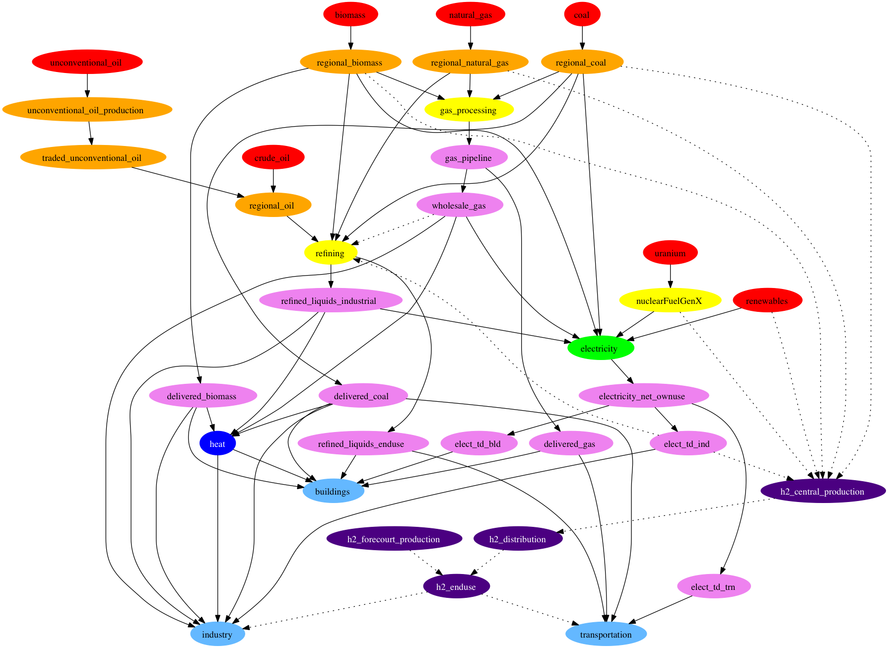
Simplified schematic of the energy system in each region, showing the inter-sectoral flows of energy goods in GCAM.
Electricity
The nesting structure of the electric sector is shown in the figure below, with a focus on one repesentative technology.
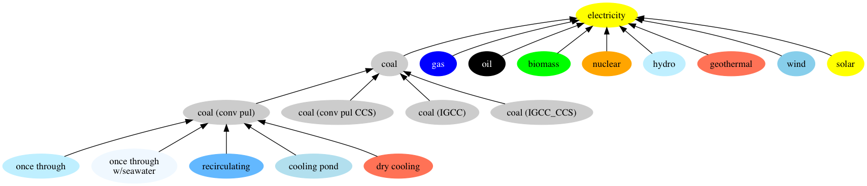
Schematic showing the nesting structure of the electric sector, with levels for choices between fuels, technologies, and cooling systems. Note that this is a simplification of the actual structure used, which includes “pass-through” sectors.
Details on the assumptions used in GCAM (e.g., cost, efficiency, capacity factors, etc.) are documented in Inputs for Modeling Supply. GCAM also includes the water inputs to electricity generation, in a third nest, as shown in the figure above. That is, within any thermo-electric generation technology, there is modeled competition between up to five different cooling system types; this is documented in the water demand section.
Refining
The structure of refining in the broader energy system is shown in the following figure, with example input-output coefficients.
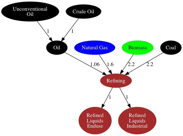
Structure of refining sector and associated products within the energy system, with sample input-output coefficients shown. Electricity and natural gas inputs to oil refining not shown for simplicity.
Oil Refining
In a typical region, the oil refining technology consumes three energy inputs: crude oil, natural gas, and electricity. This is depicted graphically below, with typical input-output coefficients shown.
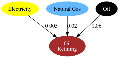
Oil refining production technology, with example coefficients.
Biomass Liquids
The biomass liquids subsector includes up to eight technologies in each region, with a global total of 11, listed in Table 1.
Table 1: Biomass liquids production technologies in GCAM
| Technology | Inputs |
|---|---|
| biodiesel (soybean) | OilCrop, natural gas |
| biodiesel (oil palm) | PalmFruit |
| biodiesel (Jatropha) | biomassOil |
| cellulosic ethanol | biomass |
| cellulosic ethanol CCS level 1 | biomass |
| cellulosic ethanol CCS level 2 | biomass |
| corn ethanol | Corn, natural gas, electricity |
| sugar cane ethanol | SugarCrop |
| FT biofuels | biomass |
| FT biofuels CCS level 1 | biomass |
| FT biofuels CCS level 2 | biomass |
Gas Processing
The structure of the natural gas supply and distribution in GCAM is shown below:
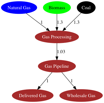
Gas processing and distribution, with example coefficients.
Note that in this structure, biogas and coal gas compete for market share of the “gas processing” market, which is upstream of the gas pipeline and distribution sectors. This structure is intended to allow for substitution away from natural gas as the feedstock for the gaseous fuels used by the energy transformation and consumption sectors, as determined by the relative economics.
Note however that the following sectors consume natural gas upstream of the network shown in the figure above: unconventional oil production, gas-to-liquids refineries, and central hydrogen production. The gas used by these three processes is not assigned the cost mark-ups or upstream pipeline losses assumed in other industrial or energy sector consumers, and there is no capacity for the model to supply the gas used for these purposes with coal- or biomass-derived gas.
District Services
In regions where purchased heat accounts for a large share of the final energy use, GCAM does include a representation of district heat production, with four competing technology options, shown below.
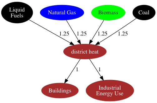
District heating structure, with example input-output coefficients shown.
As shown, all energy losses and cost mark-ups incurred in transforming primary energy into delivered district heat are accounted in the “district heat” technologies; there are no explicit cost adders and efficiency losses for heat distribution, or different prices for the heat consumed by buildings and industry sectors. This simplistic representation reflects the lack of data on district heating globally, and that the delineation of what constitutes a “third party sale” as opposed to on-site use is often unclear. This is illustrated further in the graphic below.
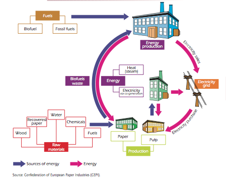
Energy flows in the pulp and paper industries, illustrating the delineation between energy producers and energy consumers. These components may or may not be located on the same property, or owned by the same entity, and the physical flows themselves often include backflows of combustible wastes from the “consumers” to the “producers”. This complicates the accounting of what constitutes a “third party” sale of heat. Source: IEA (2007)
Another accounting issue that pertains to district heating is that the regions where it is represented also tend to have a large share, up to 100% in some years, of their district heat produced at “main activity CHP plants”, which are modeled in the electricity sector in GCAM (see IEA Mapping). These are combined heat and power facilities whose primary purpose is sale of heat and/or electricity to third parties. In regions where heat is modeled as an energy commodity, the heat output of these main activity CHP plants is treated as a secondary output, and added to the total district heat produced in the given region. In future years, any new installations in the power sector are not assigned this secondary output of district heat; over time, these two sectors are modeled separately.
Hydrogen
Structure of hydrogen transmission, distribution and end use, with illustrative input-output coefficients (GJ of energy input per GJ of hydrogen) showing the approximate energy requirements of each stage of hydrogen compression, refrigeration, transportation, and storage, is shown in the figure below.
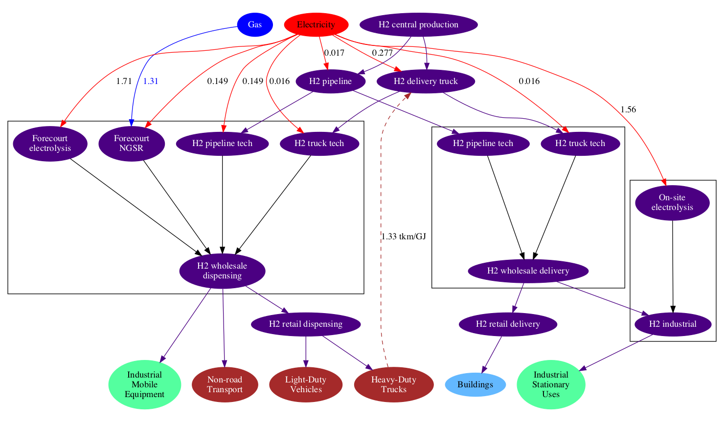
Hydrogen structure, with example input-output coefficients shown.
The most common hydrogen production technology today is natural gas steam reforming, though coal chemical transformation is the dominant technology in China IEA 2007. In GCAM, all regions have access to all technologies when hydrogen as an energy carrier becomes available; hydrogen can be produced from up to 7 primary energy sources. Three of these sources (coal, gas, and biomass) include production technologies with CCS, characterized by higher costs and higher energy intensities, but lower CO2 emissions.
Direct wind and solar electrolysis are specifically disaggregated from grid-based electrolysis because these uses of wind and solar energy do not incur any backup-related costs, unlike in the electricity sector where backup costs increase as a function of their share of total grid capacity (see electricity). Compared with grid-based electrolysis, these technologies also avoid the cost markups of electricity transmission and distribution. Each region’s costs of wind- and solar-based electrolysis are based on region-specific renewable resource supply curves and capacity factors, as well as the levelized cost of the electrolyzers, which are similarly a function of the renewable capacity factors. The nuclear technology represents thermal splitting, which does not use electricity as an intermediate energy product.
Hydrogen produced centrally can be distributed through two means: pipeline and liquefied hydrogen truck. The electricity and freight trucking input-output coefficients of each pathway are based on Argonne’s Hydrogen Delivery Scenario Analysis Model (HDSAM) ANL 2015, and reflect the respective requirements for refrigeration, compression, transportation, and storage by each distribution pathway. For end users, further energy may be required for additional compression and/or refrigeration, depending on the pathway. For example, vehicles use hydrogen that is at a higher pressure than the pipeline distribution network, and the additional on-site compression energy requirements of the dispensing stations is part of the electricity input-output coefficient to wholesale dispensing. Dispensing is generally used for hydrogen that is held at high pressure and/or low temperatures for end-use purposes (e.g., vehicles and other mobile applications), whereas delivery is used for stationary sources where storage volume is not as constrained (e.g., buildings and industrial facilities). Forecourt (i.e., on-site) production is represented as natural gas and electricity-based technologies within the delivery and dispensing sectors. These technologies typically have high levelized costs than the corresponding central technologies, due to lower capacity factors and smaller scales, but do not incur the cost markups and energy requirements of the distribution system.
Trade
Fossil fuel trade
The figure below depicts the fossil fuel trade structures (using coal as an example). In previous versions of GCAM, every region produced and consumed from a single global market. All crude oil, coal, and natural gas production was sent to a shared market, from which, every region consumed. Only net trade could be tracked and supply was affected by global rather than regional demand. The current structure maintains a global market (e.g. traded coal), but distinguishes between direct consumption of domestic resources and consumption of imported fossil fuels.
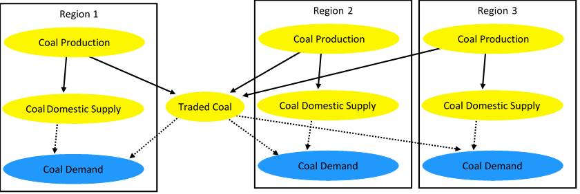
Schematics of the structures for the flows of the “Coal” commodity in GCAM, with only 3 regions shown for simplicity.
Natural gas trade
Natural gas has been further disaggregated into traded pipeline gas and traded liquefied natural gas (LNG). LNG is traded at the global market level, while pipeline gas is traded in 6 regional markets: North America, Latin America, Europe, Russia+, Africa and Middle East, and Asia-Pacific (see figures). Each GCAM region will export to only one of the regional pipeline markets, but can potentially import from multiple. The choice to have each region export from only one network is largely driven by convenience / simplicity; the pipeline networks a given region can import from is informed by bilateral UN Comtrade data on country-level gas trade (see the following section).
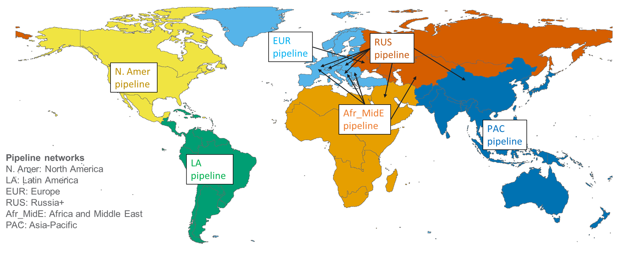
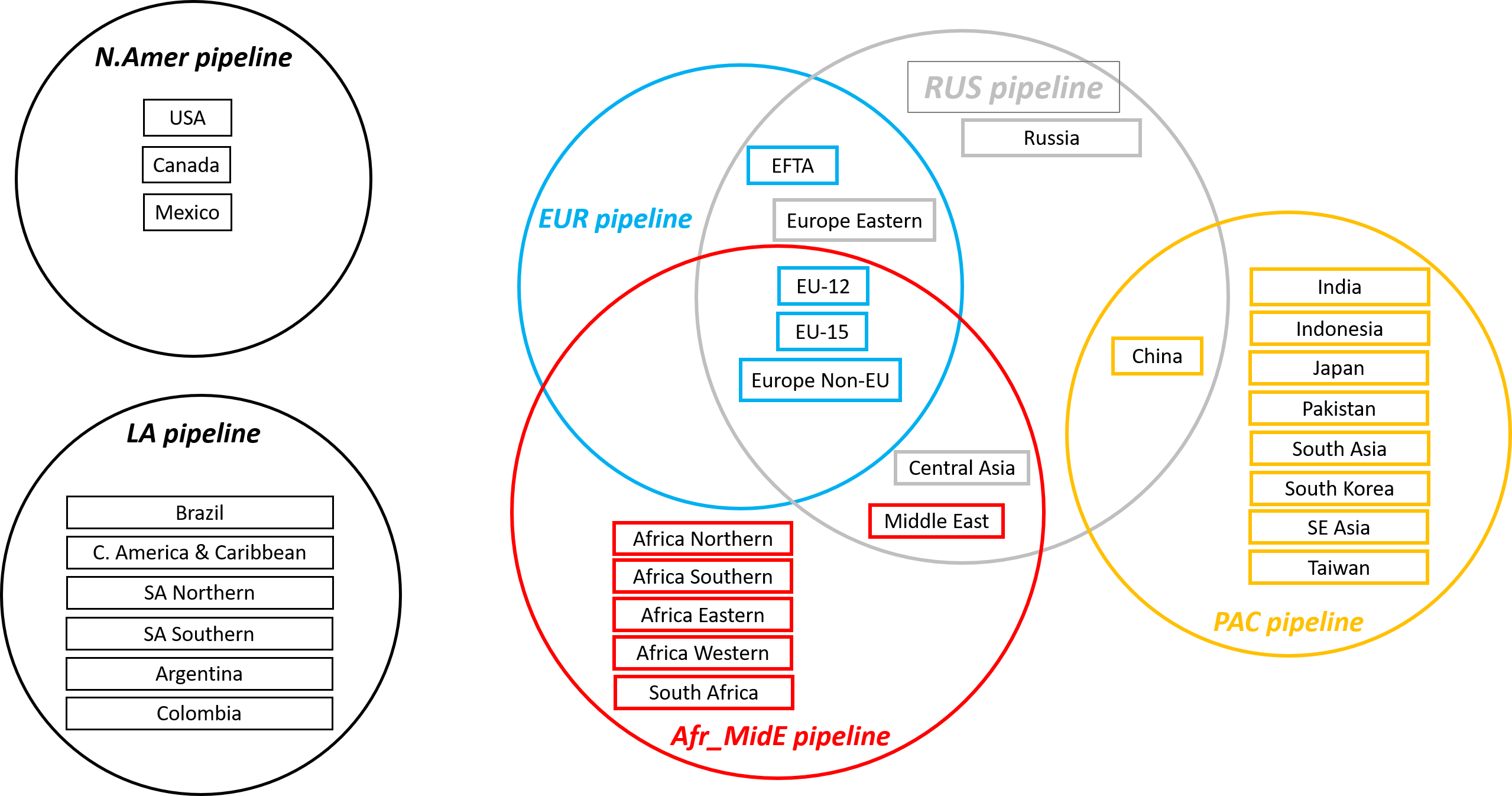
Regional gas pipeline networks. Western hemisphere (N.Amer and LA) pipeline networks are isolated. Eastern hemisphere networks partially overlap. Arrows on the map indicate additional pipeline networks that specific regions may import from, in addition to its own. Regions are located in the circles for the pipeline networks from which they import (up to 3). The boxes for each region are color coded to match the primary network that region is a part of (i.e., the one it exports to).
Data calibration for fossil fuel trade
Each region’s share of the global (e.g. traded coal) market as well as the split for domestic and imported goods are calibrated in the final base year. IEA’s data set cannot be used to make this calibration because it lacks a bilateral trade accounting. Instead the GCAM data system uses the UN’s Comtrade data set to account for intraregional trade to avoid double counting any gross trade. For example trade done within an aggregated GCAM region (e.g. Germany trading with France, both of which are in GCAM’s EU-15 region) should not be counted as part of that region’s gross trade. The Comtrade trade data is used to calculate gross trade for each region. This is then combined with the data on production and consumption of fossil fuels calculated within the data system (production is calculated from the fossil fuel supply curves and IEA data and consumption is initialized from IEA energy balances) to compute trade balances.
Energy for water
Water Flow Volumes
The historical water flow volumes for several of the sectors and processes are estimated in the water demand module, but even still several modifications are made. Table 2 shows the specific methods of estimation of each modeled water sector and process in the model, as well as the sectors from which base-year energy is re-allocated, and how the demands for each of these water flow volumes are driven in the future time periods.
Table 2: Methods of estimation of water flow volumes by EFW sectors and processes
| Sector | Process | Historical data source | Energy deducted from | Future demand driver |
|---|---|---|---|---|
| Desalinated water | Treatment | FAO Aquastat | Industry Sector; Commercial and Public Services | Municipal water demand; manufacturing water demand |
| Irrigation water | Abstraction | Irrigation water withdrawals, plus upstream distribution losses 1 | Agriculture; Commercial and Public Services | Irrigation water demand |
| Industry | Abstraction | Industrial water withdrawals, minus desalinated water use 2 | Industry Sector | Industrial Output |
| Industry | Treatment | Industrial water withdrawals, minus desalinated water use 2 | Industry Sector | Industrial Output |
| Industry | Wastewater Treatment | Industrial water withdrawals, times wastewater treatment share 3 | Industry Sector | Industrial Output |
| Municipal | Abstraction | Municipal water withdrawals, minus desalinated water use 2 | Commercial and Public Services | Municipal water demand |
| Municipal | Treatment | Municipal water withdrawals, minus desalinated water use 2 | Commercial and Public Services | Municipal water demand |
| Municipal | Distribution | Municipal water withdrawals | Commercial and Public Services | Municipal water demand |
| Municipal | Wastewater Treatment | Municipal water withdrawals, times wastewater treatment share 3 | Commercial and Public Services | Municipal water demand |
1: Upstream conveyance losses are from the nation-level estimates of Rohwer et al. 2007.
2: Historical desalinated water production is assigned to municipal and industrial consumers on the basis of the relative shares of each sector’s water withdrawal volumes
3: Historical shares of wastewater treatment are estimated as the respective sector’s withdrawal volume, minus consumptive uses, times the region’s wastewater treatment shares, estimated by nation in Liu et al. 2016. In the future these shares increase with per-capita GDP, similar to the representation of pollutant emissions abatement in the Emissions module.
Energy Intensities
With the exception of water abstraction, the energy intensities by sector and process used in GCAM are equal across all regions, and are equal to the 50th percentile of the energy intensities, first published in Liu et al. 2016 and later re-published with slight modifications in Table S3 of Kyle et al. (2021). The inter-regional variation in abstraction-related energy intensity comes from region- and sector-specific shares of groundwater versus surface water. The values are shown in Table 3.
Table 3: Assumed Energy Intensities by process
| Sector | Process | Fuel | Energy Intensity (kWh per \(m^3\)) |
|---|---|---|---|
| Desalinated water | Reverse osmosis | Electricity | 2.75 |
| Desalinated water | Thermal distillation | Natural gas or liquid fuels | 58.3 |
| Irrigation water | Abstraction - surface water | Electricity | 0.079 |
| Irrigation water | Abstraction - ground water | Electricity | 0.185 |
| Industry | Abstraction - surface water | Electricity | 0.079 |
| Industry | Abstraction - ground water | Electricity | 0.185 |
| Industry | Treatment | Electricity | 0.178 |
| Industry | Wastewater Treatment | Electricity | 0.775 |
| Municipal | Abstraction - surface water | Electricity | 0.079 |
| Municipal | Abstraction - ground water | Electricity | 0.185 |
| Municipal | Treatment | Electricity | 0.235 |
| Municipal | Distribution | Electricity | 0.247 |
| Municipal | Wastewater Treatment | Electricity | 0.597 |
Electricity used for non-renewable groundwater pumping is represented in future periods, using exogenous supply curves that have been constructed from simulated groundwater pumping over an 80 year period in Superwell (Niazi et al., 2024). The methods used are documented in (Niazi et al., 2024), Turner et al. 2019 and Kyle et al. (2021). From the Superwell output, supply curves are constructed for each GCAM region and water basin that consist of 20 “graded” points, each of which is assigned a total quantity of water, a non-energy-related cost of well construction and operation, and an electricity input-output coefficient. The grades are binned according to estimated total cost, using exogenous electricity prices; due to changes in electricity prices over time, the relative total costs of these grades may change over time (Niazi et al., 2025).
Optional Exogenous Floorspace
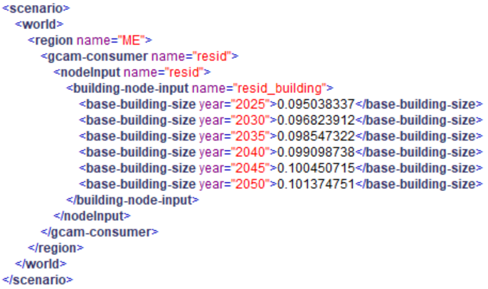
If the base assumptions are not desired, user-specified residential or commercial building floorspace values (in billion m2) can be added in a .csv file that is outside that datasystem. An XML can be generated from this .csv through Model Interface using the following header:
Floorspace, world/+{name}region, region/+{name}gcam-consumer, gcam-consumer/+{name}nodeInput, nodeInput/+{name}building-node-input,
building-node-input/+{year}base-building-size, building-node-input/+base-building-size, scenario, scenario/world
The figure below is an example XML of user-specified residential floorspace values for Maine.
References
[ANL 2015] Argonne National Laboratory, 2015, Hydrogen delivery scenario analysis model (HDSAM), Argonne National Laboratory. Link
[Denholm 2008] Denholm, P. 2008. Supply Curves for Rooftop Solar PV-Generated Electricity for the United States, Technical Report NREL/TP-6A0-44073, National Renewable Energy Laboratory. Link
[Eurek et al. 2017] Eurek, K., P. Sullivan, M. Gleason, D. Hettinger, D. Heimiller, A. Lopez (2017). An improved global wind resource estimate for integrated assessment models. Energy Economics, 64.
[IEA 2007] International Energy Agency, 2007, Tracking Industrial Energy Efficiency and CO2 Emissions, International Energy Agency, Paris, France. Link
[IHA 2000] International Hydropower Association, et al., 2000, Hydropower and the World’s Energy Future. Link
[Kyle et al. 2016] Kyle, P., Johnson, N., Davies, E., Bijl, D.L., Mouratiadou, I., Bevione, M., Drouet, L., Fujimori, S., Liu, Y., and Hejazi, M. 2016. Setting the system boundaries of “energy for water” for integrated modeling. *Environmental Science & Technology 50(17), 8930-8931. Link
[Kyle et al. 2021] Kyle, P., Hejazi, M., Kim, S., Patel, P., Graham, N., and Liu, Y. 2021. Assessing the future of global energy-for-water. Environmental Research Letters 16(2), 024031. Link
[Liu et al. 2016] Liu, Y., Hejazi, M., Kyle, P., Kim, S., Davies, E., Miralles, D., Teuling, A., He, Y., and Niyogi, D. 2016. Global and Regional Evaluation of Energy for Water. Environmental Science & Technology 50(17), 9736-9745. Link
[Niazi et al. 2024] Niazi, H., Wild, T. B., Turner, S. W. D., Graham, N. T., Hejazi, M., Msangi, S., Kim, S., Lamontagne, J. R., & Zhao, M. 2024. Global peak water limit of future groundwater withdrawals. Nature Sustainability, 7(4), pp. 413–422. Link
[Niazi et al. 2025] Niazi, H., Ferencz, S. B., Graham, N. T., Yoon, J., Wild, T. B., Hejazi, M., Watson, D. J., and Vernon, C. R. 2025. Long-term hydro-economic analysis tool for evaluating global groundwater cost and supply: Superwell v1.1. Geoscientific Model Development, 18(5), pp. 1737-1767. Link
[Rohwer et al. 2007] Rohwer, J., Gerten, D., and Lucht, W. 2007. Development of Functional Irrigation Types for Improved Global Crop Modelling. PIK Report No. 104, Potsdam Institute for Climate Impact Research. Link
[Sanders and Webber 2012] Sanders, K., and Webber, M. 2012. Evaluating the energy consumed for water use in the United States. Environmental Research Letters 7(3), 0034034. Link
[Turner et al. 2019] Turner, S.W.D., Hejazi, M., Yonkofski, C., Kim, S.H., and Kyle, P. 2019. Influence of groundwater extraction costs and resource depletion limits on simulated global nonrenewable water withdrawals over the twenty-first century. Earth’s Future 7, 123-135. Link
[Zhang et al. 2010] Zhang, Y., SJ Smith, GP Kyle, and PW Stackhouse Jr. (2010) Modeling the Potential for Thermal Concentrating Solar Power Technologies Energy Policy 38 pp. 7884–7897. Link