GCAM v8.2 Documentation: Inputs for Modeling Supply
Documentation for GCAM
The Global Change Analysis Model
View the Project on GitHub JGCRI/gcam-doc
Inputs for Modeling Supply
GCAM’s supply inputs include information on production, prices, technology cost and performance, and other emissions in the historical period in order to calibrate model parameters. In addition, GCAM’s supply modeling requires information on future technology cost and performance and emissions factors for future periods. GCAM requires that supply data is globally consistent with demand data for each of its historical model periods as it solves for market equilibrium in these years as it does for future years. These inputs are required for each region and historical year.
Table of Contents
External Inputs
Energy
Description
Table 1: External inputs used for supply of energy1
| Name | Description | Type | Source | Resolution | Unit |
|---|---|---|---|---|---|
| Historical supply of energy | Supply of energy in the historical period; used for initialization/calibration of GCAM | External data | IEA | Specified by fuel, transformation sector, country, and year | ktoe and GWh |
| CO2 capture rates | Fraction of CO2 captured in CCS technologies. | Assumption | Specified by technology and year | unitless | |
| Retirement rules | For vintaged technologies, GCAM requires the user to specify the lifetime, and the parameters required for phased and profit-based shutdown. | Assumption | Specified by technology and year | Years (for lifetime), unitless for others | |
| Logit exponents | GCAM requires the user to specify the logit exponents that determine the substitutability between technologies. | Assumption | Specified by sector and subsector | N/A | |
| Share weight interpolation rules | These rules dictate how share weights (GCAM’s calibration parameter) are specified in future years. | Assumption | Specified by subsector and technology | N/A | |
| Cost of conversion technologies | Cost of production for conversion technologies | External data | Various | Specified by technology and year | 1975$/GJ |
| Capital cost | Overnight capital cost of electricity generation technologies | External data | Annual Technology Baseline (ATB) 2019 | Specified by technology and year | 1975$/kW |
| Fixed O&M costs | Fixed operating and maintenance (O&M) costs for electricity generation technologies | External data | Annual Technology Baseline (ATB) 2019 | Specified by technology and year | 1975$/kW/yr |
| Variable O&M costs | Variable operating and maintenance (O&M) costs for electricity generation technologies | External data | Annual Technology Baseline (ATB) 2019 | Specified by technology and year | 1975$/MWh |
| Capacity factor | Ratio of generation to capacity for electricity generation technologies | Assumption | Specified by technology and year | Unitless | |
| Fixed charge rate | Factor used to levelize capital cost | Assumption | Specified by technology | Unitless | |
| Default efficiencies | Default amount of output produced per unit of input; can be overwritten by region-specific information derived from historical data | Assumption | Specified by technology and year | GJ per GJ | |
| Default input-output coefficients | Default amount of input required per unit of output produced; can be overwritten by region-specific information derived from historical data | Assumption | Specified by technology and year | GJ per GJ | |
| Resource supply curves | Mapping between cost and resource extraction. Resource extraction is cumulative for deplatable resources and annual for renewable resources | External data | Various | Specified by resource and year | EJ for extraction, 1975$/GJ for cost |
| Historical non-CO2 emissions | Historical emissions of non-CO2 | External data | CEDS v_2021_04_21 |
Specified by country, technology, gas, and year | Various |
| CO2 emissions coefficients | Default carbon content of fuels | External data | CDIAC and IEA | Specified by fuel | kgC / GJ |
| Historical CO2 emissions | Historical emissions of CO2 | External data | CDIAC | Specified by nation and year | ktC per year |
Note that for the Shared Socioeconomic Pathways (SSPs), different inputs are used for some variables. See SSPs for more information.
Data
Throughout GCAM, the number in the name of assumption file indicates to which sector the file applies. Files with A10 through A20 in the name are assumptions for resources. Files with A21 and A22 in the name are assumptions for refining and gas processing. Files with A23 in the name are assumptions for electricity, A24 is for heat, and A25 is for hydrogen. Files with A26 in the name are assumptions for transmission and distribution. Files with A61 in the name are assumptions about carbon storage.
Historical supply of energy
GCAM uses IEA energy balances as a source for historical energy supply and demand. IEA data are proprietary and thus are not provided in the GCAM data repository. Instead, we provide all of the R code used to process the IEA data so that the user can replicate the processing if they purchase the IEA data. In addition, we provide aggregated data after it has undergone processing so that GCAM input files can be created and used by the user community.
CO2 capture rates
CO2 capture rates for refining are specified in A22.globaltech_co2capture.csv. Capture rates for electricity generation are specified in A23.globaltech_co2capture.csv; capture rates for hydrogen production are specified in A25.globaltech_co2capture.csv.
Retirement rules
Retirement rules are specified in A22.globaltech_retirement.csv, A23.globaltech_retirement.csv, A25.globaltech_retirement.csv, and A10.ResSubresourceProdLifetime.csv.
Logit exponents
Logit exponents are specified in A21.sector.csv, A21.subsector_logit.csv, A22.sector.csv, A22.subsector_logit.csv, A23.sector.csv, A23.subsector_logit.csv, A24.sector.csv, A24.subsector_logit.csv, A25.sector.csv, A25.subsector_logit.csv, A26.sector.csv, A26.subsector_logit.csv, A61.subsector_logit.csv, A_ff_RegionalSector.csv, and A_ff_RegionalSubsector.csv, and A_ff_TradedSector.csv.
Share weight interpolation rules
Share weight interpolation rules are specified in A21.subsector_shrwt.csv, A21.subsector_interp.csv,
A21.tradedtech_shrwt.csv,
A21.globaltech_shrwt.csv, and
A21.globaltech_interp.csv. Similar files are defined for other sectors. For each sector, the file that ends _interp specifies the rule (e.g., fixed, linear) and the file that ends _shrwt indicates the value to interpolate to (if needed). Files that include subsector in the name define share weights at the subsector level, while globaltech, tradedtech, and globaltranTech indicate share weight information at the technology level.
Costs
Costs of conversion technologies are specified in A21.globaltech_cost.csv, A22.globaltech_cost.csv, A24.globaltech_cost.csv, A25.globaltech_cost.csv,
A26.globaltech_cost.csv, A21.globalrsrctech_cost.csv, and A61.globaltech_cost.csv.
For electricity generation technologies, costs inputs are specified in capital cost, fixed operating & maintenance costs, and variable operating & maintenance cost.
Default efficiencies
Efficiencies are specified in A23.globaltech_eff.csv, A25.globaltech_eff.csv, and A26.globaltech_eff.csv.
Default input-output coefficients
Coefficients are specified in A21.globaltech_coef.csv, A22.globaltech_coef.csv, A24.globaltech_coef.csv, A25.globaltech_coef.csv, A21.globalrsrctech_coef.csv, and A61.globaltech_coef.csv.
Resource supply curves
Resource supply curves are specified for fossil fuels, uranium, rooftop PV, EGS, geothermal, municipal solid waste , traditional biomass, onshore wind and offshore wind.
Emissions
Default carbon contents of fuels are specified in A_PrimaryFuelCCoef.csv. Historical CO2 emissions are provided in CDIAC_CO2_by_nation.csv.
Historical non-CO2 emissions information is provided in the GCAM release as “pre-built” data aggregated to GCAM regions, technologies, and fuels. Users that want to build using CEDS raw data, for example to build for different regional aggregations, will need to generate CEDS data using the open-source CEDS system and place the resulting emissions data by country, fuel, and sector within the CEDS folder.
Water
Description
Table 2: External inputs used for supply of water 2
| Name | Description | Type | Source | Resolution | Unit |
|---|---|---|---|---|---|
| Surface water supply curves (cost and availability) | Xanthos derived total maximum runoff values, combined with accessible water calculation to determine water available at very low price and the level of accessible water for cost-curve inflection | Exogenous Data | Xanthos output | Water basin and year | \(km^3\) available per USD |
| Groundwater supply curves (cost and availability) | Amount of groundwater available in each basin at increasingly high graded levels | Niazi et al., 2025; Turner et al., 2019a | Water basin and year | \(km^3\) available per USD | |
| Desalination cost | Cost of desalinated water within a basin which is available at high cost and available once the price of water within a basin surpasses a certain threshold | Exogenous Data | Global Constant | USD per \(km^3\) |
Note that for the Shared Socioeconomic Pathways (SSPs), different inputs are used for some variables. See SSPs for more information.
Data
Surface water supply curves
Surface water supply curves are based on runoff estimates from Xanthos, a detailed global hydrology model (Liu et al. 2018; Vernon et al. 2019). Xanthos accounts for surface and subsurface processes to compute runoff at 0.5° grid resolution. Global climate datasets are utilized in conjunction with Xanthos to determine historical annual average runoff aggregated for each basin (Liu et al. 2018; Turner et al., 2019a; Vernon et al. 2019). Of the total basin runoff, water available or accessible for human use takes into consideration requirements for ecosystem services, inaccessibility due to rapid flow and remote locations, and capacity of reservoir storage. Accessible fractions of total runoff vary across basins. Renewable water volumes up to the accessible fraction is available at nominal or low cost. Additional renewable water beyond the accessible fraction is available at a sharply higher cost to ensure availability of water for ecosystem services and to reflect capital investments necessary for reservoir expansion. Basin level runoff is specified in xanthos_basin_runoff.csv. Accessible fraction is specified in xanthos_accessible_water.csv. For additional accessible calculations, basin historical basin level demands are specified in basin_water_demand_1990_2015.csv and groundwater availability is specified in groundwater_trend_watergap.csv.
Groundwater supply curves
Non-renewable groundwater supply curves are modeled as a graded depletable resource with a fixed amount of total groundwater availability. Basin level estimates of environmentally exploitable groundwater are aggregated from grid-scale data (Niazi et al., 2025). Groundwater supply curves represent the relationship between exploitable groundwater and cost of extraction Niazi et al., 2024;. As the available water within the initial grades is exhausted, the price for additional groundwater resources increases as a function of depth and geological complexity. Energy inputs and costs required for pumping are included for a rigorous estimate of the relationship between groundwater volume and extraction cost (Turner et al., 2019a; Kim et al. 2016). Graded groundwater availability is specified in groundwater_constrained.csv with groundwater extraction trends found in groundwater_trend_watergap.csv and groundwater_trend_gleeson.csv.
Desalination costs
The costs of desalinated water reflects electrical energy input and capital and operational costs. Due to the high cost of desalination, desalinated water is only utilized when renewable and non-renewable water supplies are scarce and the cost of freshwater is high. Desalinated water representation is nested within the water distribution sectors where it competes with basin water supply from renewable and nonrenewable sources.
Food, Feed, and Forestry
Description
Table 3: External inputs used for supply of food, feed, and forestry 3
| Name | Description | Type | Source | Resolution | Unit |
|---|---|---|---|---|---|
| Historical country-level production of crops | Production of agricultural commodities by country in the historical period; used for initialization/calibration of GCAM | External data | FAO, gcamdata-faostat | Specified by crop, country, and year | tons |
| Historical country-level harvested area for crops | Harvested area for agricultural commodities by country in the historical period; used for initialization/calibration of GCAM | External data | FAO, gcamdata-faostat | Specified by crop, use, country, and year | ha |
| Historical sub-national production of crops | Production of agricultural commodities by water basin in a single year; used for initialization/calibration of GCAM | External data | moirai | Specified by crop, country and basin | tons |
| Historical sub-national harvested area of crops | Harvested area of agricultural commodities by water basin in a single year; used for initialization/calibration of GCAM | External data | moirai | Specified by crop, country and basin | ha |
| Historical production of livestock | Production of livestock commodities in the historical period; used for initialization/calibration of GCAM | External data | FAO, gcamdata-faostat | Specified by crop, use, country, and year | tons |
| Livestock feed coefficients | Livestock feed input, animal output, and meat output by systems | External data | IMAGE, | Specified by commodity, feed system, IMAGE region and year | various |
| Historical cost of production | Historical cost of crop production in the USA | External data | USDA | Specified by crop, type of cost, and year | various (e.g., $ per planted acre, $ per bushel) |
| Historical prices | Historical prices of agriculture and livestock commodities; used for initialization/calibration of GCAM | External data | FAO, gcamdata-faostat | Specified by country, commodity, and year | |
| Agriculture productivity growth | Projected yields through 2050 for agricultural commodities | External data | FAO | Specified by country, commodity, and year | |
| Logit exponents | Share parameters dictating substitution between different feed options for livestock | Assumption | Specified by type of livestock | unitless | |
| Historical non-CO2 emissions | Historical emissions of non-CO2 | External data | CEDS v2024_07_08 |
Specified by country, technology, gas, and year | Various |
Note that for the Shared Socioeconomic Pathways (SSPs), different inputs are used for some variables. See SSPs for more information.
Data
Historical production and harvested area
For both production and harvested area of crops, GCAM blends country level time series provided by the FAO with subnational information provided by moirai in a single year to determine historical production and harvested area for each GCAM land region. FAO data is specified in GCAMFAOSTAT_NonFodderProdArea.csv.gz and GCAMFAOSTAT_FodderProdArea.csv.gz. Moirai data is specified in LDS_ag_prod_t.csv and LDS_ag_HA_ha.csv. Livestock production is specified along with the supply utilization accounts in GCAMFAOSTAT_SUA.csv.gz.
Livestock feed information
GCAM bases its historical livestock feed representation on the IMAGE model. GCAM utilizes information from IMAGE v3.1 on the animal feed by system, animal head by system, and animal meat production.
Ag productivity growth
GCAM captures change in yield due to increases in fertilizer use or irrigation endogenously. All other non-climate related factors driving yield increases are exogenously specified, with data specified in FAO_ag_CROSIT.csv.
Prices
GCAM uses producer prices to initialize the model (future prices are endogenous). Those prices are provided in GCAMFAOSTAT_ProdPrice.csv.gz.
Cost of production
The costs associated with land, irrigation, and fertilizer are endogenously determined in GCAM (see Land Supply). Other costs of production are exogenously specified and the data used for those costs can be found in USDA_cost_data.csv, with USDA_item_cost.csv specifying which costs are included in GCAM. Note that we use cost information for the USA in all regions.
Emissions
Historical non-CO2 emissions information is provided in the GCAM release as “pre-built” data aggregated to GCAM regions, technologies, and fuels. Users that want to build using CEDS raw data, for example to build for different regional aggregations, will need to generate CEDS data using the open-source CEDS system and place the resulting emissions data by country, fuel, and sector within the CEDS folder.
gcamfaostat
There has been a significant data method update for the GCAM AgLU (Agriculture and Land Use) sectors in GCAM v7, which is described in detail in CMP #360. An additional package (gcamfaostat; Zhao et al. 2024) is developed to facilitate the processing of data from FAOSTAT in a transparent, traceable, and consistent manner. This update encompasses the following key advancements:
- Functions have been developed to automate the updating of AgLU data, primarily sourced from FAOSTAT. This automation facilitates future updates to advance the model’s final historical period and allows for other data adjustments to be easily incorporated. Note that most of the data in the
aglu/FAOfolder are now generated by gcamdata-faostat. - The new update incorporates the compilation of FAO FBS (food balance sheet) and SUA (supply-utilization accounting) data. This integration enables the tracing of flows from land-based primary production to end uses, both in terms of food and non-food purposes. It provides a comprehensive understanding of the agricultural supply and demand.
- New methods have been developed to generate “primary equivalent,” which serves as a bridge between primary agricultural supply and final consumption. This calculation helps to bridge the gap between the production of agricultural commodities and their ultimate utilization in various forms.
The aggregation of agricultural data from FAO countries and commodities to GCAM regions and commodities are included in gcamdata. The commodity mapping is provided in Mapping_SUA_PrimaryEquivalent.csv and shown in the following Figures for crop harvested area and food availability.
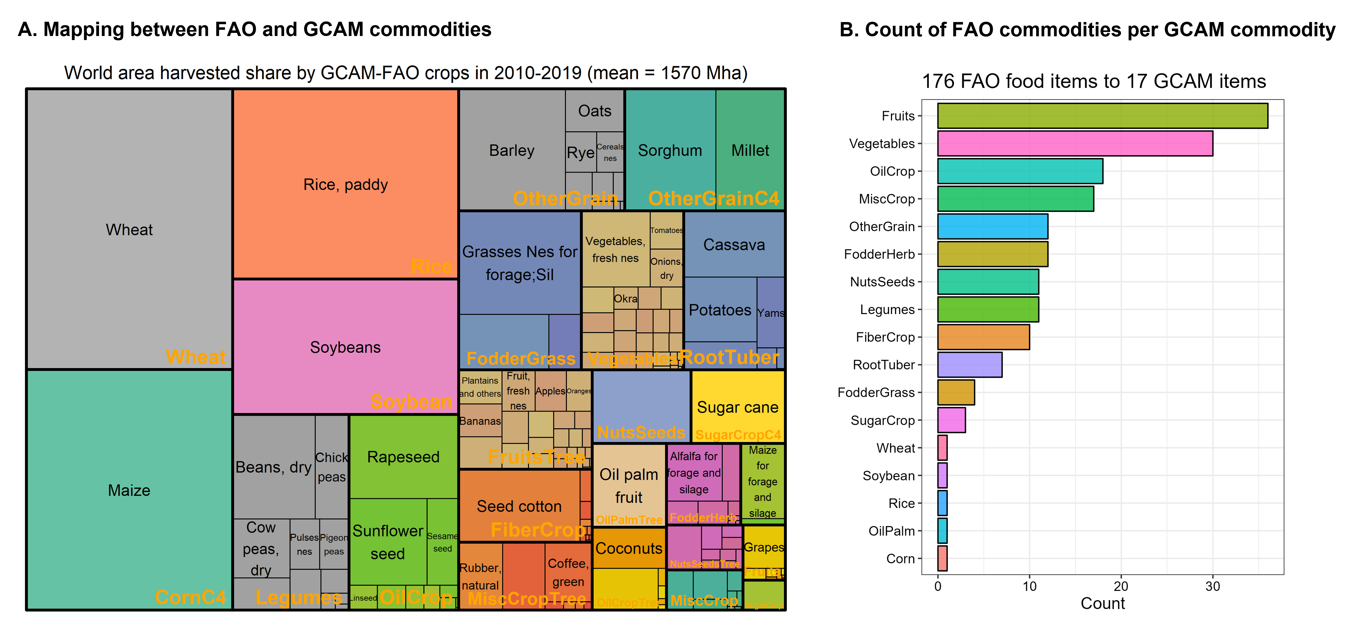
Mapping between FAO and GCAM primary (land-based) commodities (A) and count of FAO commodities per GCAM commodity (B)
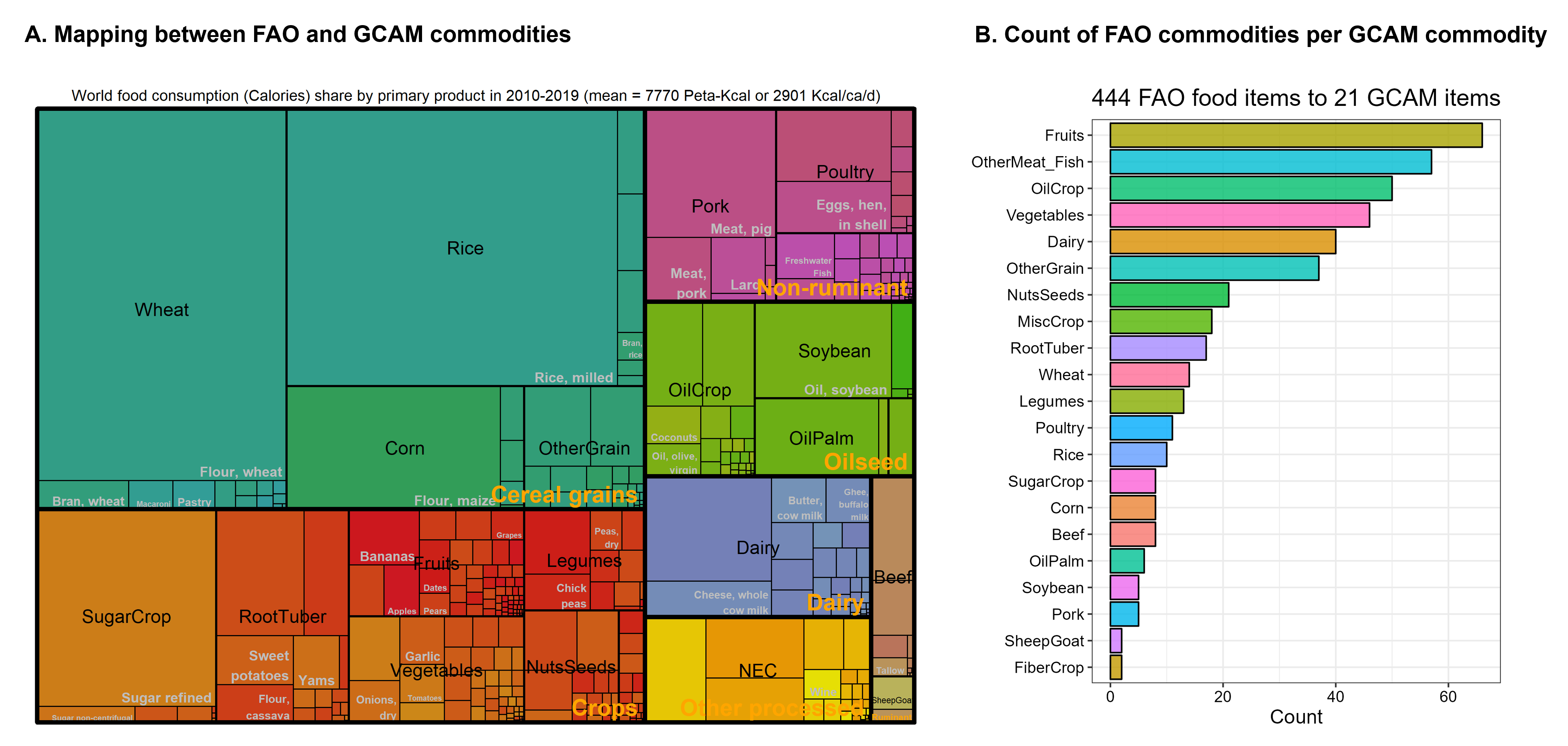
Mapping between FAO and GCAM food commodities (A) and count of FAO commodities per GCAM commodity (B)
In GCAM v7.1, leveraging the newly compiled SUA data, we separated opening stock, closing stock, and the corresponding storage loss.
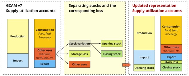
Schematic of the restructuring of the supply-utilization accounts in GCAM to separate agricultural storage and the corresponding loss
References
[CDIAC 2017] Boden, T., and Andres, B. 2017, National CO2 Emissions from Fossil-Fuel Burning, Cement Manufacture, and Gas Flaring: 1751-2014, Carbon Dioxide Information Analysis Center, Oak Ridge National Laboratory. Link
[IEA 2023] International Energy Agency, 2023, Energy Balances of OECD Countries 1960-2022 and Energy Balances of Non-OECD Countries 1971-2022, International Energy Agency, Paris, France.
[Kim et al. 2016] Kim SK, Hejazi M, et al. (2016). Balancing global water availability and use at basin scale in an integrated assessment model. Climatic Change 136:217-231. Link
[Kyle et al. 2021] Kyle, P., Hejazi, M., Kim, S., Patel, P., Graham, N., & Liu, Y. (2021). Assessing the future of global energy-for-water. Environmental Research Letters, 16(2), 024031.
[Liu et al. 2018] Liu Y., M. Hejazi, H. Li, X. Zhang, G. Leng (2018). A hydrological emulator for global applications - HE v1.0.0. Geoscientific Model Development. Link
[Niazi et al. 2024] Niazi, H., Wild, T. B., Turner, S. W. D., Graham, N. T., Hejazi, M., Msangi, S., Kim, S., Lamontagne, J. R., & Zhao, M. 2024. Global peak water limit of future groundwater withdrawals. Nature Sustainability, 7(4), pp. 413–422. Link
[Niazi et al. 2025] Niazi, H., Ferencz, S. B., Graham, N. T., Yoon, J., Wild, T. B., Hejazi, M., Watson, D. J., and Vernon, C. R. 2025. Long-term hydro-economic analysis tool for evaluating global groundwater cost and supply: Superwell v1.1. Geoscientific Model Development, 18(5), pp. 1737-1767. Link
[Turner et al. 2019a] Turner S.W.D., M. Hejazi, C. Yonkofski, S. Kim, P. Kyle (2019a). Influence of groundwater extraction costs and resource depletion limits on simulated global nonrenewable water withdrawals over the 21st century. Earth’s Future (2019), 10.1029/2018EF001105 Link
[Vernon 2019] Vernon, C., M. Hejazi, S. Turner, Y. Liu, C. Braun, X. Li, and R. Link. A Global Hydrologic Framework to Accelerate Scientific Discovery. Journal of Open Research Software (2019). Link
[Zhao 2024] Zhao, Xin, Maksym Chepeliev, Pralit Patel, Marshall Wise, Katherine Calvin, Kanishka Narayan, and Chris Vernon. “gcamfaostat: An R package to prepare, process, and synthesize FAOSTAT data for global agroeconomic and multisector dynamic modeling.” Journal of Open Source Software 9, no. 96 (2024): 6388.