Fldgen v2 Tutorial - Joint Temperature and Precipitation emulation and function how to • fldgen

The fldgen package allows you to ingest temperature and precipitation output from an earth system model (ESM) and generate randomized temperature fields that have the same space and time correlation properties as the original ESM data. This tutorial focuses on how to use the functions in the package to generate and analyze joint temperature and precipitation fields. The details of how the method works are covered in a companion paper.

All of the functions used here are documented in R’s help system. Since our purpose here is to outline what functions have to be called, and in what sequence, to perform the analysis, we haven’t repeated material from the help files. If you’re confused about how a function is supposed to work, consult the help files. For example, help(read.temperatures) will print the docs for the function that reads the netCDF temperature fields.

Using the field generator

Setup

## parameters for the code below.
ngen <- 4             # number of fields to generate
nplt <- ngen          # number of fields to plot
exfld <- 20           # example field to plot from the time series
set.seed(8675309)     # Set RNG seed so results will be reproducible

All of the data needed for this tutorial is installed with the package.

library('fldgen')
datadir <- system.file('extdata', package='fldgen')

One-step emulator training

You can do the read and analyze steps below in a single command by running:

infileT <- file.path(datadir, 'tas_annual_esm_rcp_r2i1p1_2006-2100.nc')
infileP <- file.path(datadir, 'pr_annual_esm_rcp_r2i1p1_2006-2100.nc')
emulator <- trainTP(c(infileT, infileP), 
                    tvarname = "tas", tlatvar='lat_2', tlonvar='lon_2',
                    tvarconvert_fcn = NULL,
                    pvarname = "pr", platvar='lat', plonvar='lon',
                    pvarconvert_fcn = log)

If you want to use multiple ESM runs for the training (recommended), you can either pass trainTP a list of filenames, or you can give it the name of a directory, in which case it will use all of the netCDF files it finds there. trainTP will automatically pair temperature (tas) amd precipitation (“pr”) annual average netcdf files based on the file name (CMIP5 convention) and only train the emulator on paired files.

For the fldgen method to work, each ESM variable must be able to accept residuals of between infinity and -infinity. This is already the case for temperature and no transformation is needed (tvarconvert_fcn = NULL). Because precipitation cannot be less than 0, either the generated residuals have to be constrained to avoid negative precipitation while preserving the ESM spatiotemporal statistics, or the method must operate on a transformation of precipitation that can accept residuals between -infinity and infinity. The latter is more straightforward, and so residuals are generated for log(precipitation) rather than precipitation (pvarconvert_fcn = log). Any function that is continuous, invertible, and monotonic and results in a transformed variable supported on (-infinity, infinity) will preserve the ESM spatiotemporal statistical properties as desired.

For users that wish to customize the training process, a detailed explanation of the science in each step is included in this vignette.

One-step residual field generation

You can generate any number of residual fields in a single command (shown for generating 3 fields):

residgrids <- generate.TP.resids(emulator, ngen = 3)

residgrids is a list of ngen entries, each containing a matrix of residuals [Ntime X 2Ngrid] for a single realization. Columns 1:Ngrid contain the temperature residuals for the realization. Columns (Ngrid+1):2Ngrid contain the precipitation residuals for the realization.

With the default inputs to trainTP, tvarconvert_fcn = NULL and pvarconvert_fcn = log, the residuals will be generated in (temperature, log(precipitation)) space.

One-step full field construction

This can also be accomplished in one command:

fullgrids <- generate.TP.fullgrids(emulator, residgrids,
                                   tgav = emulator$tgav,
                                   tvarunconvert_fcn = NULL, 
                                   pvarunconvert_fcn = exp,
                                   reconstruction_function = pscl_apply)

Note that the inclusion of the argument pvarunconvert_fcn = exp means that the full grids are provided in (temperature, precipitation) space. The log(precipitation) transformation has been undone. Also note that for the tgav argument we have passed in the tgav stored in the emulator structure; however, we could just as readily have passed in any future pathway for global mean temperature that we wanted to investigate.

The science of each step

Setup (repeated)

## parameters for the code below.
ngen <- 4             # number of fields to generate
nplt <- ngen          # number of fields to plot
exfld <- 20           # example field to plot from the time series
set.seed(8675309)     # Set RNG seed so results will be reproducible

All of the data needed for this tutorial is installed with the package.

library('fldgen')
datadir <- system.file('extdata', package='fldgen')

Reading the ESM data

The ESM temperature and precipitation fields should be in netCDF files. The function that reads it returns a griddata structure that contains the data, as well as some information about the grid, such as the latitude, longitude, and time coordinates and the vector of area weights needed to compute grid averages.

filenameT <- file.path(datadir, 'tas_annual_esm_rcp_r2i1p1_2006-2100.nc')
griddataT <- read.general(filenameT,
                          varname='tas', latvar='lat_2', lonvar='lon_2',
                          timevar='time')
tgav <- griddataT$vardata %*% griddataT$globalop


filenameP <- file.path(datadir, 'pr_annual_esm_rcp_r2i1p1_2006-2100.nc')
griddataP <- read.general(filenameP,
                          varname='pr', latvar='lat', lonvar='lon',
                          timevar='time')

Here, we have read in the temperature netCDF data and used the global average operator to compute a time series of global mean temperatures. We have also read in the precipitation netCDF data. These variables will be used as input to the functions that analyze the ESM data and produce the joint temperature and precipitation fields. Next we must define the transformation functions, as described above. Temperature doesn’t need one, but for precipitation we will use a log transformation so that we can ensure that output precipitation values are >= 0.

tvarconvert_fcn <- NULL
pvarconvert_fcn <- log

    # make sure supported on -infinity to infinity, add some output data to
    # facilitate the reversing later
    if(!is.null(tvarconvert_fcn)){
        griddataT$vardata_raw <- griddataT$vardata
        griddataT$vardata <- tvarconvert_fcn(griddataT$vardata)
    } else {
        griddataT$vardata_raw <- NULL
    }
    griddataT$tvarconvert_fcn <- tvarconvert_fcn

    if(!is.null(pvarconvert_fcn)){
        griddataP$vardata_raw <- griddataP$vardata
        griddataP$vardata <- pvarconvert_fcn(griddataP$vardata)
    } else {
        griddataP$vardata_raw <- NULL
    }
    griddataP$pvarconvert_fcn <- pvarconvert_fcn

# the temperature and precipitation data must be on the same grid size:
ncol(griddataT$vardata) ==  ncol(griddataT$vardata)
#> [1] TRUE

Ngrid <- as.numeric(ncol(griddataT$vardata))

Analyzing the input data

The first thing we need is a model for the mean temperature response in each grid cell and a model for the mean precipitation response in each grid cell. That is, for each grid cell, what is the mean temperature of that cell as a function of global mean temperature. For each grid cell, what is the mean precipitation in that grid cell as a function of global mean temperature. You can use whatever model you want for this. We will use a simple linear pattern scaling model, which is implemented in the pscl_analyze function.

This package could subsititute any variable that scales with global mean temperature for precipitaiton, to generate joint temperature and (arbitrary variable) fields. Some labels remaining to precipitation may persist though, and this is currently considered an unsupported use of the package.

psclT <- pscl_analyze(griddataT$vardata, tgav)

psclP <- pscl_analyze(griddataP$vardata, tgav)

The mean response analysis should return the model coefficients (called w and b in our linear model) and a time series of gridded residuals. These residuals encode all of the information about the spatial variability of the ESM.

One key feature of the method used in fldgen is that, due to the Central Limit Theorem, any residuals that it generates for a grid cell will be normally distributed. While temperature residuals are approximately normally distributed in each grid cell, this is not the case for precipitation residuals. Further, principal component analysis, a key step of the the empirical orthogonal functions (EOF) analysis, has the nicest properties when it is provided with normally distributed inputs.

Therefore, we empirically characterize the distribution of residals in each grid cell with a custom empirical cdf and its inverse (custom empirical quantile function).

tfuns <- characterize.emp.dist(psclT$r)
pfuns <- characterize.emp.dist(psclP$r)

A custom empirical cdf is constructed for each grid cell because the R function for producing an empirical cdf, ecdf, produces a step function that is, by definition, neither continuous nor invertible. The custom empirical cdf in each grid cell produced by characterize.emp.dist is instead piecewise linear, creating a continous invertible function, tfuns$cdf. For convenience, characterize.emp.dist also pre-computes the inverse tfuns$quant.

These empirical distributions in each grid cell are then used to map the residuals from their native (ESM) distribution to $N(0,1)$ via quantiles. Consider a temperature residual value, $r$ in grid cell $n$. Then tfuns$cdf[[n]](r) will map the temperature residual value to the its quantile value. This quantile value is then input to qnorm to give a corresponding normal residual value from $N(0,1)$.

normresidsT <- normalize.resids(inputresids = psclT$r,
                                empiricalcdf = tfuns$cdf)$rn
normresidsP <- normalize.resids(inputresids = psclP$r,
                                empiricalcdf = pfuns$cdf)$rn

This transformation from native to normal space is continuous, invertible, and monotonic. Therefore, in additionn to being reversible (so that we can transform generated fields back to the native space), this transformation preserves the rank (first place = largest, last place = smallest) of residuals within a grid cell. Because the rank of residuals in any grid cell $n$ is the same in the native space as it is in the normal space, the Spearman correlation coefficient between any pair of grid cells $m,n$ is the same in the native space as the normal space. Therefore, the transformation from native to normal space (or normal to native space) preserves the spatial structure of residuals. In particular, this works for comparing the spatial structure of temperature residuals with temperature residuals, temperature residuals with precipitation residuals, and precipitation residuals with precipitation residuals. The transformation performed by normalize.resids (and the inverse process unnormalize.resids) is constructed to truly preserve the joint spatial structure of temperature and precipitation.

These normally distributed residuals are passed to the empirical orthogonal functions (EOF) analysis. Specifically, they are passed as a joint matrix of (transformed) temperature and preciptiation residuals. Therefore, the EOFs are each vectors with 2Ngrid entries, forming an orthonormal basis for the space of joint temperature and precipitation residuals. Essentially, this is the state of the system at some particular time - a large vector that contains every temperature residual in every grid cell, followed by every precipitation residual in every grid cell.

reof <- eof_analyze(as.matrix(cbind(normresidsT, normresidsP)),
                    Ngrid = Ngrid, globop = griddataT$globalop)

The next thing we need to generate our fields is the temporal structure of the EOF coefficients. We get this from the Fourier transform of the coordinates of the residuals in the coordinate system defined by the EOF basis vectors.

Fx <- mvfft(reof$x)
Fxmag <- abs(Fx)
Fxphase <- atan2(Im(Fx), Re(Fx))

Finally, we need to create an array of coefficients for some constraint equations that our generated fields need to satisfy.

phasecoef <- phase_eqn_coef(Fx)

The functions for generating fields will expect the results of these calculations to be packaged in an object like the one returned from trainTP. There is a function for taking our hand generated results and turning them into an object.

infiles <- list(filenameT, filenameP)
emulator <- fldgen_object_TP(griddataT, griddataP,
                             tgav, psclT, psclP,
                             tfuns, pfuns,
                             reof, Fxmag, Fxphase,
                             infiles)

Generating residual fields - more detail

Now we’re ready to generate fields. We’ll do 4 fields in this example. The first one will be a reconstruction of the original input. The other three will be new fields with random phases. The two steps used here to generate these new fields with random phases make up the interior of generate.TP.resids() and could be replaced with a call to that function (see tests/testthat/test_varfield.R lines 199-230 for an example). Because the EOF analysis was performed on a joint matrix of transformed T and P residuals, each grid cell in a generated field follows $N(0,1)$.

newgrids <- list()
length(newgrids) <- ngen


## First field will have the same phases as the input ESM data
newgrids[[1]] <- reconst_fields(reof$rotation, mkcorrts(emulator, Fxphase))

## Other fields will have random phases
for(i in 2:ngen) {
  newgrids[[i]] <- reconst_fields(reof$rotation, mkcorrts(emulator))
}

The generated residual fields are transformed back to the native space:

## Subtract off the mean field.  Save these because we will want to use them later
residgrids <- lapply(newgrids, function(g) {
    g[, 1:Ngrid] <- unnormalize.resids(empiricalquant = emulator$tfuns$quant,
                                       rn = g[ ,1:Ngrid])$rnew

    g[, (Ngrid+1):(2*Ngrid)] <- unnormalize.resids(empiricalquant = emulator$pfuns$quant,
                                                   rn = g[ , (Ngrid+1):(2*Ngrid)])$rnew

    return(g)}
)

Creating a full field from residuals

Whether you get your list of generated residual matrices from calling generate.tp.resids() or doing manually in more detail, the mean field is reconstructed and added to each residual field and transformed back to the native ESM variable where relevant (i.e. precipiation rather than log(precipitation)) to create new, full global gridded temperature and precipitation realizations.

## Here tgav is the same as the input, but that doesn't have to be the case
meanfieldT <- pscl_apply(psclT, tgav)
meanfieldP <- pscl_apply(psclP, tgav)


tvarunconvert_fcn <- NULL
pvarunconvert_fcn <- exp

   lapply(residgrids, function(matrix, gridcells = Ngrid){

        # Separate the tas and pr data from one another.
        tas <- matrix[ , 1:Ngrid]
        pr  <- matrix[ , (Ngrid + 1):(2 * Ngrid)]

        # Add the meanfield to the data
        tas[ , 1:Ngrid] <- tas[ , 1:Ngrid] + meanfieldT
        pr[ , 1:Ngrid]  <- pr[ , 1:Ngrid] + meanfieldP

        # convert from (-inf, inf) support to natural support.
        if( !is.null(emulator$griddataT$tvarconvert_fcn)){

            tas <- tvarunconvert_fcn(tas)

        }

        if(!is.null(emulator$griddataP$pvarconvert_fcn)){

            pr <- pvarunconvert_fcn(pr)

        }

        # Return output
        return(list(tas = tas, pr = pr))

    }) ->
        fullgrids

Plotting the fields

We can extract a single field from each time series and plot them all for comparision. We will be able to see a lot more detail if we subtract out the mean field from each one, so that’s what we will do.

## Extract a single example field from each series and create a plot
if(dofieldplots) {
plotglobalfieldsT <- function(fieldlist, sequencenum, minval=-3.5, maxval=3.5, legendstr) {
    ## Extract a single example field from each series (sequencenum determines which one) and create a plot
    lapply(fieldlist, function(g) {
        suppressWarnings(
            plot_field(g[sequencenum, 1:Ngrid], emulator$griddataT, 14,  # 14 is the number of color levels in the plot
                       minval, maxval) +
                guides(fill=ggplot2::guide_colorbar(barwidth=ggplot2::unit(4,'in'), barheight=ggplot2::unit(0.125,'in'),
                                                    title=legendstr, title.position='top', title.hjust=0.5))
        )
    })
}

plotglobalfieldsP <- function(fieldlist, sequencenum, minval=-1.5, maxval= 1.5, legendstr) {
    ## Extract a single example field from each series (sequencenum determines which one) and create a plot
    lapply(fieldlist, function(g) {
        suppressWarnings(
            plot_field(g[sequencenum, (Ngrid + 1):(2*Ngrid)], emulator$griddataP, 14,  # 14 is the number of color levels in the plot
                       minval, maxval) +
                guides(fill=ggplot2::guide_colorbar(barwidth=ggplot2::unit(4,'in'), barheight=ggplot2::unit(0.125,'in'),
                                                    title=legendstr, title.position='top', title.hjust=0.5))
        )
    })
}


residfieldplotsT <- plotglobalfieldsT(residgrids[1:nplt], exfld, legendstr='delta-T (K)')
residfieldplotsP <- plotglobalfieldsP(residgrids[1:nplt], exfld, legendstr='delta-logP (log(kg/m2/s))')

## Display the plots
for (i in 1:length(residfieldplotsT)) {
   gridExtra::grid.arrange(residfieldplotsT[[i]], residfieldplotsP[[i]], nrow = 1)
}
} else {
  print('Unable to make plots: gcammaptools is not installed.')
}
#> [1] "Unable to make plots: gcammaptools is not installed."

EOF Characteristics

Note that the EOFs are a basis for residuals in the normal space. Because our transformations between normal and native are rank preserving, a large normal residual transforms to a large native residual.

Time behavior

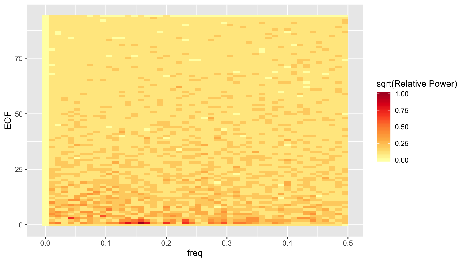
Start by constructing a heatmap of the power spectrum for the EOFs. Technically we will be plotting the square root of the power spectrum, which is fine for getting a sense of what trends exist in the data, but we’ll need to keep that in mind if we decide to do anything quantitative with the power.

nt <- length(griddataT$time)
## There is no additional information in the negative frequencies, so keep only
## the positive ones.
np <-
    if(nt %% 2 == 1) {
        (nt+1)/2
    } else {
        nt/2 + 1
    }

hmdata <- reshape2::melt(Fxmag[1:np,])
hmdata$freq <- (hmdata$Var1 - 1) / nt    # The - 1 is due to R's unit-indexed arrays.
hmdata$EOF <- as.integer(substring(hmdata$Var2, 3))
## discretize the power so we can isolate structure more easily
nbrk <- 10
hmdata$discval <- findInterval(hmdata$value / max(hmdata$value), seq(0.01, 0.99, length.out=nbrk)) / nbrk
hmdata <- dplyr::select(hmdata, EOF, freq, value, discval) %>% as_tibble()

hmplt <- ggplot(hmdata, aes(x=freq, y=EOF, fill=discval)) + geom_raster() + scale_fill_distiller(palette='YlOrRd', direction=1, name='sqrt(Relative Power)')

print(hmplt)

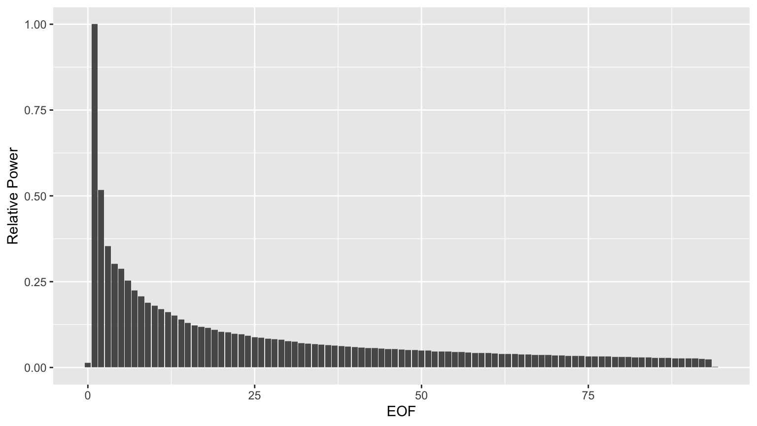
Evidently, the power drops off quite a bit after the first few EOFs.

eofpwr <- group_by(hmdata, EOF) %>% summarise(totpwr=sum(value*value)) %>% mutate(relpwr=totpwr/max(totpwr)) %>% select(EOF, relpwr)
eofpwrplt <- ggplot(eofpwr, aes(x=EOF, y=relpwr)) + geom_col() + ylab('Relative Power')
print(eofpwrplt)

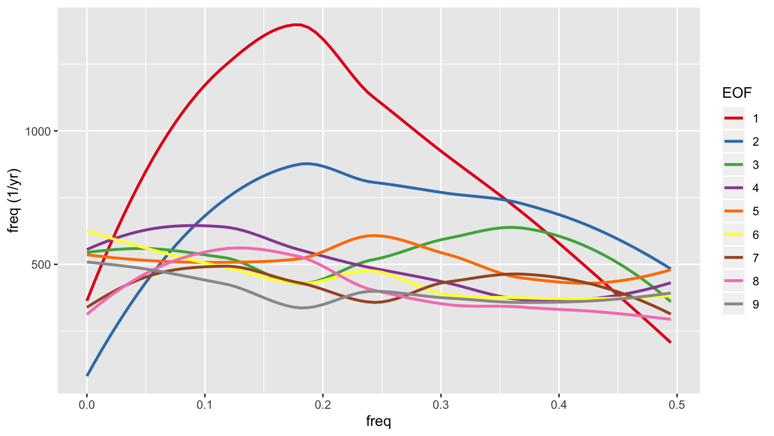
More importantly, the power spectrum whitens after the first few EOFs, so those early EOFs represent periodic signals, while the later ones don’t. Here are the smoothed power spectra for the first 9 EOFs.

eofspectra <- filter(hmdata, EOF>0, EOF<10) %>% mutate(EOF=factor(EOF))
eofspectraplt <- ggplot(eofspectra, aes(x=freq, y=value, color=EOF)) + geom_smooth(se=FALSE) + scale_color_brewer(palette='Set1') + ylab('freq (1/yr)')
print(eofspectraplt)
#> `geom_smooth()` using method = 'loess' and formula 'y ~ x'

Spatial behavior

We will make spatial plots of the 9 EOFs shown in the plot above. We’ll also plot EOFs 25 and 50, just to get an idea of what’s happening in those lower power modes. Note that a single EOF contains both temperature and precipitation information. We represent that information in a pair of maps - the spatial structure of the temperature EOF and the spatial structure of the precipitation EOF.

### Plotting global maps is still a little slow, so expect this to take some time.
## The EOFs are in reof$rotation.  Each column is the grid cell values for an EOF.
## Also, the EOFs are scaled to unit norm.  We'll rescale them to unit max value

if(dofieldplots) {
  eofcols <- c(2:10, 26, 51)  # EOF numbering starts at 0, but array numbering starts at 1
  eofvis <- t(reof$rotation[,eofcols])   # EOFs are now in rows, not columns
  eofvis <- eofvis / max(abs(eofvis))


  eofpltsT <- lapply(seq_along(eofcols), function(i) {
    title <- paste0('EOF-', eofcols[i]-1)
    suppressWarnings(plot_field(eofvis[i, 1:Ngrid], emulator$griddataT, 14, -0.5, 0.5)) +
        ggtitle(title) +
        guides(fill=ggplot2::guide_colorbar(barwidth=ggplot2::unit(4,'in'), barheight=ggplot2::unit(0.125,'in'),
                                                      title="T-portion (relative to max of T portion)", title.position='top',
                                            title.hjust=0.5))
    })


    eofpltsP <- lapply(seq_along(eofcols), function(i) {
        title <- paste0('EOF-', eofcols[i]-1)
        suppressWarnings(plot_field(eofvis[i, (Ngrid + 1): (2 * Ngrid)], emulator$griddataP, 14, -0.5, 0.5)) +
            ggtitle(title) +
            guides(fill=ggplot2::guide_colorbar(barwidth=ggplot2::unit(4,'in'), barheight=ggplot2::unit(0.125,'in'),
                                                      title="P-portion (relative to max of P portion)", title.position='top',
                                                title.hjust=0.5))
    })


    for(i in seq_along(eofcols)) {
        gridExtra::grid.arrange(eofpltsT[[i]], eofpltsP[[i]], nrow = 1)
    }
} else {
  print('Unable to make plots:  gcammaptools is not installed.')
}
#> [1] "Unable to make plots:  gcammaptools is not installed."

Fldgen v2 Tutorial - Joint Temperature and Precipitation emulation and function how to

Abigail Snyder

2019-03-23