ambrosia: An R package for calculating and analyzing food demand that is responsive to changing incomes and prices
Summary
The ambrosia R package was developed to calculate food demand for staples and non-staple commodities that is responsive to changing levels of incomes and prices. ambrosia implements the framework to quantify food demand as established by Edmonds et al. (2017) and allows the user to explore and estimate different variables related to the food demand system. Currently ambrosia provides three main functions:
- calculation of food demand for any given set of parameters including income levels and prices,
- estimation of calibration parameters within a given a dataset. Note:
ambrosiais used to calculate parameters for the food demand model implemented in the Global Change Analysis Model. - exploration and preparation of raw data before starting a parameter estimation.
Statement of need and audience
An important motivation to develop ambrosia is functionalizing and separating out the different components of the sophisticated food demand framework into usable R functions that can be easily parameterized and customized by the user.Thus, the tool not only enables easy use and future development, but also enables easy modularization of the code within other systems.
ambrosia has been developed to help researchers explore questions related to trends in food demand empirically. Since the equations of the model are grounded in peer reviewed research while the code itself is written in R (which increases usability), the tool is useful to researchers interested in,
1) analyzing and exploring trends in food demand with a computational model that is responsive to changes in incomes and prices that can easily be implemented on any time series (dataset); 2) re-estimating calibration parameters of the food demand model using custom data, thus effectively allowing the user to calibrate the model to custom data; 3) incorporating a detailed food demand model in their own earth system and economic models.
Getting Started with ambrosia
ambrosia can be directly installed from its GitHub repository using the R devtools package. From an R prompt, run the command,
devtools::install_github('JGCRI/ambrosia', build_vignettes = TRUE)User tutorial and examples
A list of examples along with a user tutorial describing the different features in ambrosia are available in the ambrosia_vignette. To load the vignette with examples for the major functions within ambrosia, run the following command
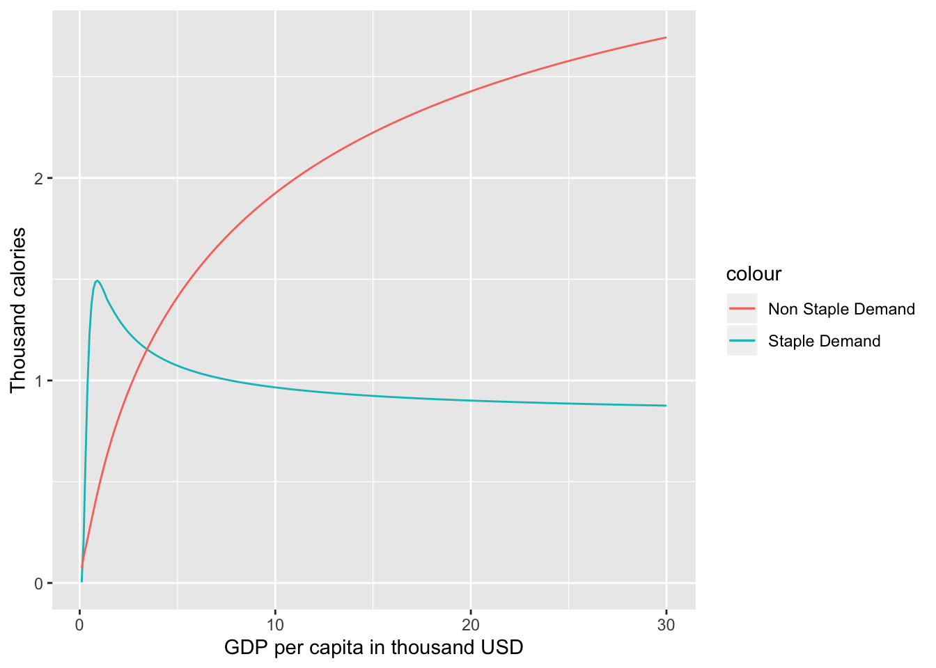
vignette("ambrosia_vignette")The example below shows how a user can get an estimate of demand using some sample parameters (See the table below for description of parameters).
#Get a sample data set
Test_Data <- data.frame(Y=seq(0.1,30, by=0.1))

#Add sample values of Ps and Pn
Test_Data %>% mutate(Ps=0.1,Pn=0.2) -> Test_Data

#Now calculate food demand
Food_Demand <- food.dmnd(Test_Data$Ps, Test_Data$Pn, Test_Data$Y)
The code from the example can be used to visualize the food demand for staples and non-staples as follows,
Description of calibration parameters
The 11 calibration parameters are described in table below with values from the latest version of ambrosia. The table also contains an acceptable range for each of the parameters. The original parameters were calculated using a Markov Chain Monte Carlo (MCMC) approach. The range is calculated as the 95% Joint Confidence Interval of the range of the parameters apperaing in all Monte Carlo samples with likelihood values above the 5th percentile.Parameters in the table below are calibrated on the basis of national level data on food consumption and food consumption prices for staples and non-staple products.
| Parameter name | Description | Units | Value | Range of parameter values |
|---|---|---|---|---|
A_s |
A scale term used to derive expenditure share for staple demand | Unitless | 1.28 | 1.25 -1.40 |
A_n |
A scale term used to derive expenditure share for non-staple demand. | Unitless | 1.14 | 0.9 - 1.16 |
xi_ss |
Price elasticity of staple goods. Unit change in per capita demand for staples as a result of unit increase in price (in $ per person per day). | Elasticity | -0.19 | -0.27 - -0.07 |
xi_cross |
Cross price elasticity between staples and non-staples which in combination with the other price elasticities is used to derive substitution elasticity. | Elasticity | 0.21 | 0.09 - 0.27 |
xi_nn |
Price elasticity of non-staple goods. Unit change in per capita demand for non-staples as a result of unit increase in price (in $ per person per day). | Elasticity | -0.3 | -0.46 - -0.10 |
nu1_n |
Income elasticity for non-staple goods. Unit change in per capita demand for non-staples for unit change in income (in thousand USD). | Elasticity | 0.5 | 0.46 - 0.61 |
lambda_s |
Income elasticity for staple goods. Unit change in per capita demand for staples for unit change in income (in thousand USD) | Elasticity | 0.1 | 0.075 - 0.16 |
k_s |
Log of Income level at which staple demand is anticipated to be at its highest | Thousand USD | 16 | 10 -17 |
psscl |
Additional scaling term used to derive the expenditure shares for staples. This is applied to price of staples (Ps/Pm * psscl), where Ps is the price of staples and Pm is the price of materials and to the expenditure shares of staples (alpha_s). |
Unitless | 100 | 80 - 120 |
pnscl |
Additional scaling term used to derive the expenditure shares for non-staples. This is applied to price of non-staples (Pn/Pm * pnscl), where Pn is the price of non-staples and Pm is the price of materials and to the expenditure shares of non-staples (alpha_n). |
Unitless | 20 | 18 - 25 |
Pm |
Price of materials (everything else in the economy other than food products) | $ per day | 5 | 2 -6 |
Simple example of equations to derive demand using calibration parameters described above.
Below is a simple example of how quantities of demand for staples (Q_s) and non-staples (Q_n) in thousand calories are calculated using the above 11 calibration parameters above for an income level of Y in thousand USD for a staple price of Ps in $ per calorie per day and non-staple price of Pn in $ per calorie per day.
# 1) Staple demand

Q_s <- A_s * Ps ^ xi_ss * Pn ^ xi_cross * Income_Term_staples

where,

Income_term_staples <- (k_s * Y) ^ (lambda_s / Y)

Pn <- Pn/Pm

Ps <- Ps/Pm

# 2) Non-staple demand

Q_n <- A_n * Ps ^ xi_cross * Pn ^ xi_nn * Income_Term_Non_staples

where,

Income_Term_Non_staples <- Y ^ (2 * nu1_n)

Pn <- Pn/Pm

Ps <- Ps/Pm
Contributing to ambrosia
We welcome contributions to ambrosia from the development community. Please contact us at the email IDs below if you want to collaborate! The ambrosia GitHub repository is accessible here: GitHub Repository. In order to report issues with ambrosia, please open an issue in the above mentioned Github Repository.
For more information about contributing, please contact Kanishka Narayan at kanishka.narayan@pnnl.gov or Chris Vernon at chris.vernon@pnnl.gov
Availability
Dependencies
dplyr (>= 0.7)
nleqslv (>= 3.2)
reshape2 (>= 1.4.3)
ggplot2 (>= 2.2.1)
cluster (>= 2.0)
tidyr (>= 0.7.1)
Code repository
Name- GitHub; JGCRI/ambrosia
Identifier- https://github.com/JGCRI/ambrosia/tree/v1.3.5
License- BSD 2-Clause
