The functions that form this module take the emission sets per TM5-FASST region and year generated in Module 1 (by m1_emissions_rescale), and estimate the fine particulate matter (PM2.5) and ozone (O3) concentration levels for each period and TM5-FASST region. In particular the package reports the following range of PM2.5 and O3 indicators:
Fine particulate matter (PM2.5) concentration levels (m2_get_conc_pm25)
library(rfasst)
library(magrittr)

 db_path<-"path_to_your_gcam_database"
 query_path<-"path_to_your_gcam_queries_file"
 db_name<-"name of the database"
 prj_name<-"name for a Project to add extracted results to" # (any name should work, avoid spaces just in case)
 scen_name<-"name of the GCAM scenario"
 queries<-"Name of the query file" # (the package includes a default query file that includes all the queries required in every function in the packae, "queries_rfasst.xml")
 saveOutput: Writes the files.By default=T
 map: Produce the maps. By default=F

  # To write the csv files into the output folder:

     m2_get_conc_pm25(db_path,query_path,db_name,prj_name,scen_name,queries,saveOutput=T,map=F)

  # To save as data frame pm2.5 concentration levels by TM5-FASST region in year 2050:

     pm25.conc.2050<-dplyr::bind_rows(m2_get_conc_pm25(db_path,query_path,db_name,prj_name,scen_name,queries,saveOutput=F)) %>% dplyr::filter(year==2050)

head(pm25.conc.2050)- Ozone concentration levels (
m2_get_conc_o3)
library(rfasst)
library(magrittr)

 db_path<-"path_to_your_gcam_database"
 query_path<-"path_to_your_gcam_queries_file"
 db_name<-"name of the database"
 prj_name<-"name for a Project to add extracted results to" # (any name should work, avoid spaces just in case)
 scen_name<-"name of the GCAM scenario",
 queries<-"Name of the query file" # (the package includes a default query file that includes all the queries required in every function in the packae, "queries_rfasst.xml")
 saveOutput: Writes the files.By default=T
 map: Produce the maps. By default=F

  # To write the csv files into the output folder:

     m2_get_conc_o3(db_path,query_path,db_name,prj_name,scen_name,queries,saveOutput=T,map=F)

  # To save as data frame ozone (O3) concentration levels by TM5-FASST region in year 2050:

     o3.conc.2050<-dplyr::bind_rows(m2_get_conc_o3(db_path,query_path,db_name,prj_name,scen_name,queries,saveOutput=F)) %>% dplyr::filter(year==2050)

head(o3.conc.2050)- Maximum 6-monthly running average of daily maximum hourly O3 (M6M, also known as 6mDMA1) (
m2_get_conc_m6m)
library(rfasst)
library(magrittr)

 db_path<-"path_to_your_gcam_database"
 query_path<-"path_to_your_gcam_queries_file"
 db_name<-"name of the database"
 prj_name<-"name for a Project to add extracted results to" # (any name should work, avoid spaces just in case)
 scen_name<-"name of the GCAM scenario",
 queries<-"Name of the query file" # (the package includes a default query file that includes all the queries required in every function in the packae, "queries_rfasst.xml")
 saveOutput: Writes the files.By default=T
 map: Produce the maps. By default=F

  # To write the csv files into the output folder:

     m2_get_conc_m6m(db_path,query_path,db_name,prj_name,scen_name,queries,saveOutput=T,map=F)

  # To save as data frame ozone-M6M (6mDMAI) concentration levels by TM5-FASST region in year 2050:

     m6m.conc.2050<-dplyr::bind_rows(m2_get_conc_m6m(db_path,query_path,db_name,prj_name,scen_name,queries,saveOutput=F)) %>% dplyr::filter(year==2050)

head(m6m.conc.2050)- Accumulated daytime hourly O3 concentration above a threshold of 40 ppbV (AOT40) (
m2_get_conc_aot40)
library(rfasst)
library(magrittr)

 db_path<-"path_to_your_gcam_database"
 query_path<-"path_to_your_gcam_queries_file"
 db_name<-"name of the database"
 prj_name<-"name for a Project to add extracted results to" # (any name should work, avoid spaces just in case)
 scen_name<-"name of the GCAM scenario"
 queries<-"Name of the query file" # (the package includes a default query file that includes all the queries required in every function in the packae, "queries_rfasst.xml")
 saveOutput: Writes the files.By default=T
 map: Produce the maps. By default=F

  # To write the csv files into the output folder:

     m2_get_conc_aot40(db_path,query_path,db_name,prj_name,scen_name,queries,saveOutput=T,map=F)

  # To save as data frame ozone-AOT40 concentration levels by TM5-FASST region in year 2050:

     aot40.conc.2050<-dplyr::bind_rows(m2_get_conc_aot40(db_path,query_path,db_name,prj_name,scen_name,queries,saveOutput=F)) %>% dplyr::filter(year==2050)

head(aot40.conc.2050)- Seasonal mean daytime O3 concentration (
m2_get_conc_mi)
library(rfasst)
library(magrittr)

 db_path<-"path_to_your_gcam_database"
 query_path<-"path_to_your_gcam_queries_file"
 db_name<-"name of the database"
 prj_name<-"name for a Project to add extracted results to" # (any name should work, avoid spaces just in case)
 scen_name<-"name of the GCAM scenario",
 queries<-"Name of the query file" # (the package includes a default query file that includes all the queries required in every function in the packae, "queries_rfasst.xml")
 saveOutput: Writes the files.By default=T
 map: Produce the maps. By default=F

  # To write the csv files into the output folder:

     m2_get_conc_mi(db_path,query_path,db_name,prj_name,scen_name,queries,saveOutput=T,map=F)

  # To save as data frame ozone-Mi concentration levels by TM5-FASST region in year 2050:

     mi.conc.2050<-dplyr::bind_rows(m2_get_conc_mi(db_path,query_path,db_name,prj_name,scen_name,queries,saveOutput=F)) %>% dplyr::filter(year==2050)
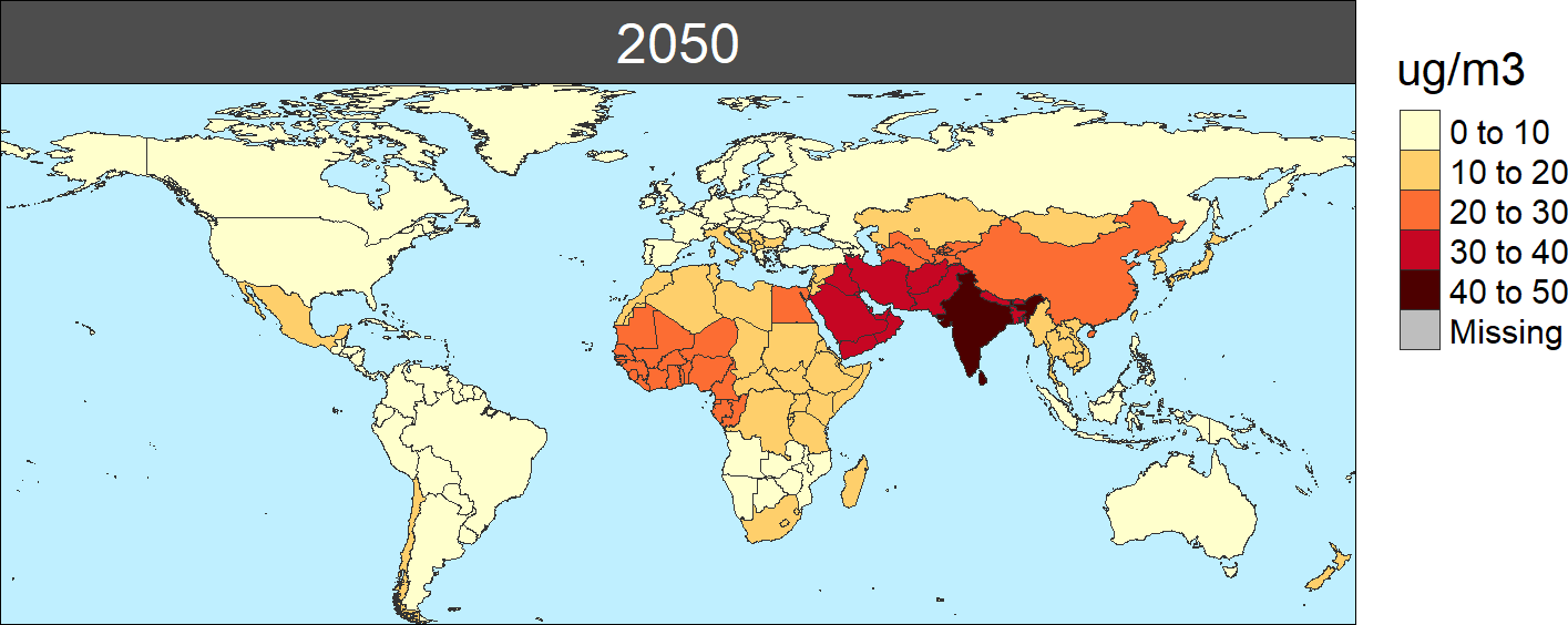
head(mi.conc.2050)map=T parameter, and they will be generated and stored in the corresponding output sub-directory. As an example for this module, the following map shows the PM2.5 concentrations in 2050:
PM2.5 concntration by region in 2050 (ug/m3)
As indicated in the documentation of TM5-FASST Van Dingenen et al 2018,estimates of PM2.5 and O3 concentration levels in a receptor region driven by the emissions of different precursors in different sources are based on parametrizations of meteorology and atmospheric chemistry drawn from the more complex TM5 model. In summary, concentration of a pollutant \(j\), in region \(y\), from all the precursors (\(i\)) emitted in all regions (\(x_k\)), is calculated as:
\[C_j (y)=C_{j,base} (y)+∑_{k=1}^{n_x}∑_{i=1}^{n_i}SRC_{i,j} [x_k,y]\cdot[E_i (x_k)-E_{i,base} (x_k )]\]
\(C_{j,base} (y)\) is the base-run concentration level of pollutant j in region y, pre-computed with TM5.
\(E_{i,base} (x_k)\) are the base-run precursor i emissions in region \(x_k\)
\(SRC_{i,j} [x_k,y]\) = the \(i\)–to-\(j\) source-receptor coefficient for source region \(x_k\) and receptor region y, pre-computed from a 20% emission reduction of component i in region \(x_k\) relative to the base-run
\(E_i (x_k)\) are the emissions of precursor i in region \(x_k\) in the analyzed scenario.
Following this equation, base-run emissions and concentrations, and source-receptor coefficient matrixes need to be combined with emissions pathways for the analyzed scenario. The package includes the following input information:
- Source-receptor coefficient matrixes (SRC):
- PM2.5 Source-receptor matrixes:
- SO4: SO2, NOx and NH3
- NO3: NOx, SO2, and NH3
- NH4: NH3, NOx and SO2
- BC: BC_POP
- POM: POM_POP
- O3 Source-receptor matrixes:
- For O3 exposure (O3): NOx, NMVOC and SO2
- For health calculations: M6M (6mDMA1): NOx, NMVOC, SO2 and CH4
- For agricultural damages:
- AOT40: NOx, NMVOC, SO2 and CH4
- Mi (M7 and M12): NOx, NMVOC, SO2 and CH4
- PM2.5 Source-receptor matrixes:
The package also includes the base emission and concentration levels for all these indicators.
In addition, primary PM2.5 emissions (BC and POM) are assumed to have a more direct influence in urban (more dense) areas, so the emission-concentration relation for these two pollutants is modified using adjustment coefficients that are included in the package.