Tutorial for the `pridr` software package, prepared for IAMC 2022

Pre-processing, loading libraries

##LOAD our package
library(pridr)


#Other packages
library(ggplot2)
library(ggsci)
library(parallel)
library(tidyr)
library(dplyr)
library(data.table)
library(assertthat)
library(viridis)
library(knitr)


#Basic format for figs (optional)
scheme_basic <- theme_bw() +
  theme(legend.text = element_text(size = 15)) +
  theme(legend.title = element_text(size = 15)) +
  theme(axis.text = element_text(size = 18)) +
  theme(axis.title = element_text(size = 18, face = "bold")) +
  theme(plot.title = element_text(size = 15, face = "bold", vjust = 1)) +
  theme(plot.subtitle = element_text(size = 9, face = "bold", vjust = 1))+ 
  theme(strip.text = element_text(size = 7))+
  theme(strip.text.x = element_text(size = 18, face = "bold"))+
  theme(strip.text.y = element_text(size = 15, face = "bold"))+
  theme(legend.position = "bottom")+
  theme(legend.text = element_text(size = 12))+
  theme(legend.title = element_text(size = 12,color = "black",face="bold"))+
  theme(axis.text.x= element_text(hjust=1))+
  theme(legend.background = element_blank(),
        legend.box.background = element_rect(colour = "black"))

Example 1: Generate deciles using lognormal approach

`We load a sample dataset with GINI coefficients and mean income (by country, year) and derive the income distribution (deciles) using the lognormal based approach.`

`1. Load a sample dataset`

read.csv("Input_Data/Wider_aggregated_deciles.csv", stringsAsFactors = FALSE) %>%
  select(country, year, gdp_ppp_pc_usd2011, gini) %>%
  distinct() %>%
  mutate(sce="Historical data") %>% 
  filter(year > 2013)->data_for_lognorm

knitr::kable(head(data_for_lognorm), format = "html")

country	year	gdp_ppp_pc_usd2011	gini	sce
Argentina	2014	18.9490	0.396005	Historical data
Australia	2014	43.5615	0.342125	Historical data
Austria	2014	43.8475	0.298130	Historical data
Austria	2015	44.0700	0.297710	Historical data
Belgium	2014	41.3035	0.274710	Historical data
Belgium	2015	41.7700	0.271340	Historical data

`2. Use the lognormal model on this dataset`

start_time= Sys.time()
compute_deciles_lognormal(data_for_lognorm)->lognormal_model

end_time=Sys.time()

print(paste0("Processed in ",as.integer(end_time-start_time), " seconds"))

## [1] "Processed in 5 seconds"

knitr::kable(head(lognormal_model), format = "html")

country	year	category	pred_shares	model
Argentina	2014	d1	0.0217603	Log normal based downscaling (using country GINI)
Argentina	2014	d2	0.0349525	Log normal based downscaling (using country GINI)
Argentina	2014	d3	0.0450210	Log normal based downscaling (using country GINI)
Argentina	2014	d4	0.0598386	Log normal based downscaling (using country GINI)
Argentina	2014	d5	0.0678814	Log normal based downscaling (using country GINI)
Argentina	2014	d6	0.0830141	Log normal based downscaling (using country GINI)

Example 2: Generate lognormal density dist (For an abritary set of parameters)

`Here, we generate lognormal density distribution from arbritary values of the GINI and mean income.`

density_dist_1 <- compute_lognormal_dist(mean_income = 15,gini=0.6) %>% mutate(gini=as.character(0.6))
density_dist_2 <- compute_lognormal_dist(mean_income = 15,gini=0.3)%>% mutate(gini=as.character(0.3))
density_dist_3 <- compute_lognormal_dist(mean_income = 15,gini=0.2)%>% mutate(gini=as.character(0.2))

g <- ggplot(data=bind_rows(density_dist_3,density_dist_2,density_dist_1), aes(x=gdp_pcap,y=density,color=gini))+
     geom_line(size =2)+scale_color_aaas()+ xlab("Income in Thous USD")

g+scheme_basic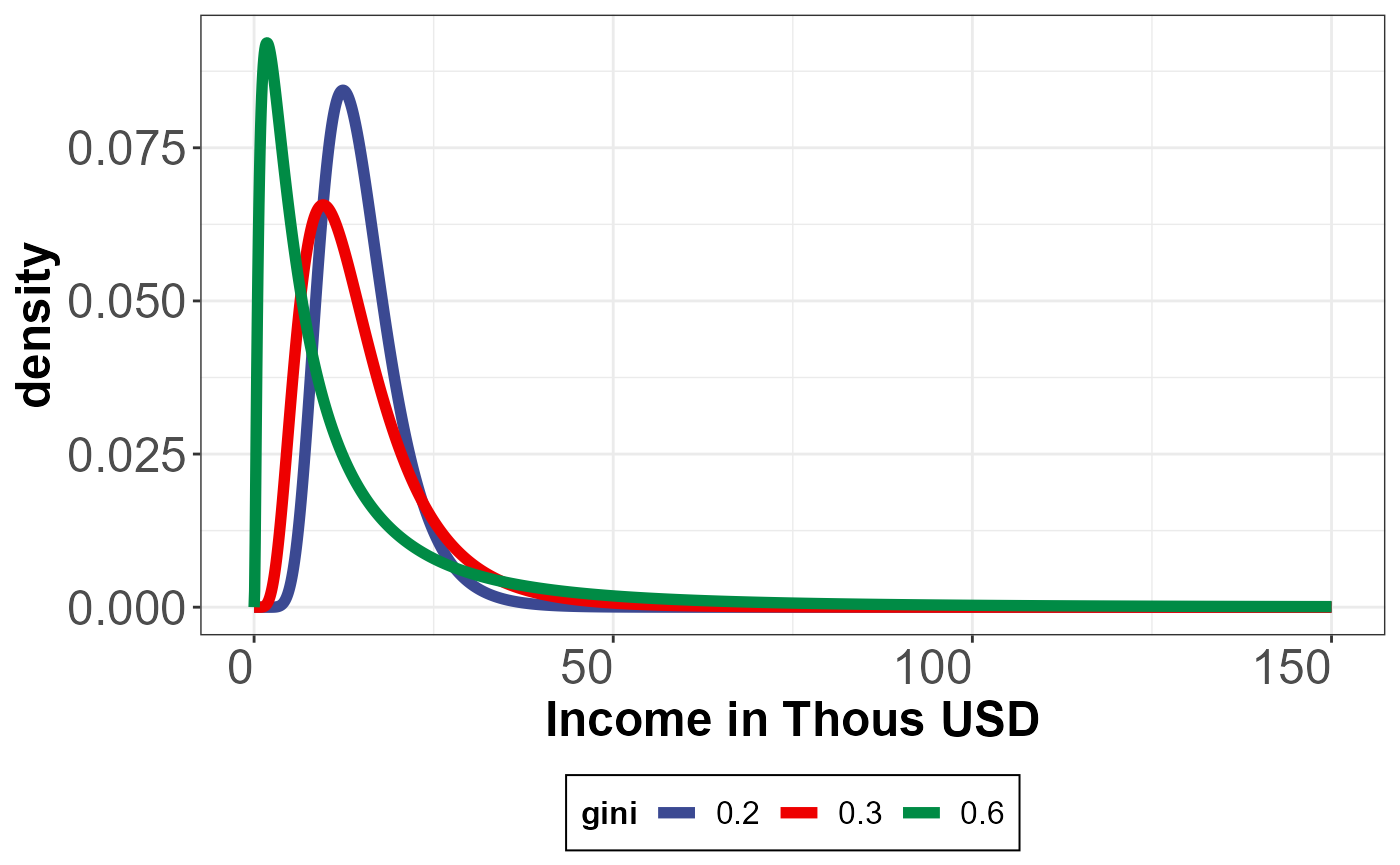

Example 3. Use the PCA based model

`Here , we demonstrate the usage of the PCA based model. We pass a dataset of required variables (Step 1 below) to the`PC_model`function (Step 2 below). Note that the function parameters are stored in memory for pridr and will not change unless the user specifically resets parameters (using newer data for example).`

`1. Compile data (This is the dataset format that needs to be passed to the function)`

sample_data <- read.csv("Input_Data/sample_data.csv")
knitr::kable(head(sample_data), format = "html")

X	country	year	iso	sce	gini	labsh	lagged_ninth_decile	lagged_palma_ratio
1	China	1977	chn	Historical data	0.1857180	0.5921686	0.1469042	0.9035953
2	China	1978	chn	Historical data	0.2115421	0.5921686	0.1469042	0.9035953
3	China	1976	chn	Historical data	0.2254473	0.5921686	0.1469042	0.9035953
4	China	1982	chn	Historical data	0.2309190	0.5921686	0.1469042	0.9035953
5	China	1980	chn	Historical data	0.2333932	0.5921686	0.1469042	0.9035953
6	China	1992	chn	Historical data	0.2353070	0.5752647	0.1480236	1.2233429

`2. Run PC model on this dataset`

start_time <- Sys.time()

PC_model_results <- PC_model(sample_data %>% filter(iso=="usa"))

## [1] "Computed all coeffcients in each time step. Now generating deciles"

print(paste0("Completed in ", as.integer(Sys.time()-start_time), " seconds."))

## [1] "Completed in 7 seconds."

knitr::kable(head(PC_model_results), format = "html")

country	year	Category	pred_shares	Component1	Component2
United States of America	2012	d1	0.0178931	2.523811	-0.9284825
United States of America	2014	d1	0.0179736	2.554260	-0.9932798
United States of America	2015	d1	0.0179853	2.480462	-0.9124102
United States of America	2011	d1	0.0180795	2.543543	-1.0198806
United States of America	2009	d1	0.0185508	2.308630	-0.9222637
United States of America	2006	d1	0.0190730	2.124993	-0.9025370

`3. Plot results`

g <- ggplot(data=PC_model_results %>% filter(year %in% c(2010:2015)) ,aes(x=factor(Category,levels =c('d1','d2','d3','d4',
  'd5','d6','d7','d8',                                                                                'd9','d10')),y=pred_shares,color=year,group=year))+
     geom_line()+
     geom_point()+scale_color_viridis()+xlab("Deciles")+
     ggtitle("Income distributions in the US in multiple years  ")

g+scheme_basic+theme(legend.position = "right")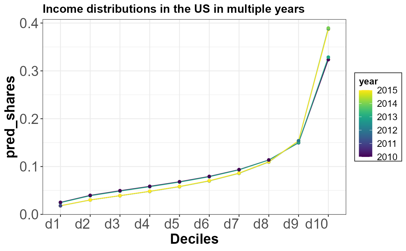

Example 4. Generate GINI coefficients for a given set of deciles

pridr`allows users to recalculate summary metrics such as the GINI coefficient from deciles.`

gini_data <-compute_gini_deciles(PC_model_results %>% mutate(category=Category), inc_col = "pred_shares",grouping_variables = c("country","year")) %>% rename(gini=output_name)
knitr::kable(head(gini_data), format = "html")

country	year	Category	pred_shares	Component1	Component2	category	share_of_richer_pop	score	gini
United States of America	2012	d1	0.0178931	2.523811	-0.9284825	d1	0.9	0.0339969	0.4660090
United States of America	2014	d1	0.0179736	2.554260	-0.9932798	d1	0.9	0.0341499	0.4666982
United States of America	2015	d1	0.0179853	2.480462	-0.9124102	d1	0.9	0.0341721	0.4646415
United States of America	2011	d1	0.0180795	2.543543	-1.0198806	d1	0.9	0.0343511	0.4662052
United States of America	2009	d1	0.0185508	2.308630	-0.9222637	d1	0.9	0.0352466	0.4588485
United States of America	2006	d1	0.0190730	2.124993	-0.9025370	d1	0.9	0.0362387	0.4528108

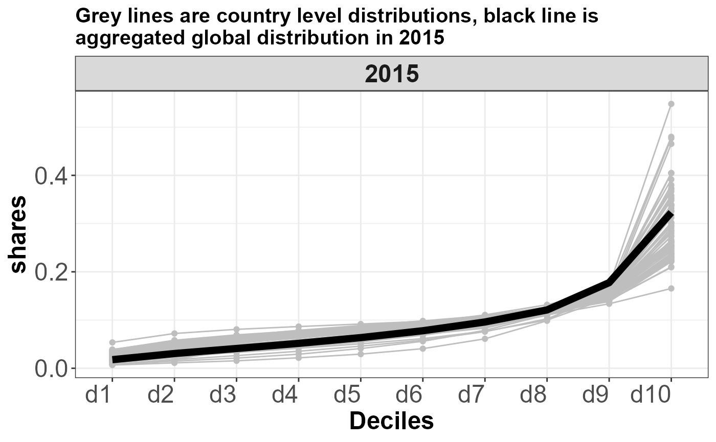
Example 5. Aggregate deciles to a region (Here we aggregate country level distributions to a global distribution)

`Users can also aggregate the income distribution to a regional or global scale based on arbritary mapping of ISOs to regions. Here, we aggregate all income distributions at the country level to a global income distribution in 2015.`

`1. Compile data`

read.csv("Input_Data/Wider_aggregated_deciles.csv", stringsAsFactors = FALSE) %>%
  select(country, year, gdp_ppp_pc_usd2011, population,Income..net.,Category) %>% filter(year%in% c(2015)) %>% mutate(GCAM_region_ID="Global")->ISO_data
knitr::kable(head(ISO_data), format = "html")

country	year	gdp_ppp_pc_usd2011	population	Income..net.	Category	GCAM_region_ID
Austria	2015	44.0700	17357324	0.0299000	d1	Global
Belgium	2015	41.7700	22575871	0.0343000	d1	Global
Bolivia	2015	6.4880	21594437	0.0111000	d1	Global
Brazil	2015	14.7535	410433868	0.0125000	d1	Global
Chile	2015	22.3865	35732037	0.0182667	d1	Global
Colombia	2015	13.0185	95749365	0.0119000	d1	Global

`2. Aggregate the distribution`

aggregate_country_deciles_to_regions(ISO_data,
                                     grouping_variables = c("GCAM_region_ID","year")
                                     )->agg_data

knitr::kable(head(agg_data), format = "html")

GCAM_region_ID	year	category	shares	gdp_pcap	tot_gdp	tot_pop	share_of_richer_pop	score	output_name
Global	2015	d1	0.0178482	14.68421	176725558262	12035076741	0.9	0.0339115	0.432179
Global	2015	d2	0.0305933	14.68421	176725558262	12035076741	0.8	0.0520086	0.432179
Global	2015	d3	0.0410385	14.68421	176725558262	12035076741	0.7	0.0615578	0.432179
Global	2015	d4	0.0516415	14.68421	176725558262	12035076741	0.6	0.0671339	0.432179
Global	2015	d5	0.0635952	14.68421	176725558262	12035076741	0.5	0.0699547	0.432179
Global	2015	d6	0.0778195	14.68421	176725558262	12035076741	0.4	0.0700376	0.432179

`3. Plot the distributions`

g <- ggplot(data=ISO_data,aes(x=factor(Category,levels =c('d1','d2','d3','d4',
  'd5','d6','d7','d8',                                                                                'd9','d10')),y=Income..net.),group=country)+
     geom_line(data=ISO_data,aes(x=factor(Category,levels =c('d1','d2','d3','d4',
  'd5','d6','d7','d8',                                                                                'd9','d10')),y=Income..net.,group=country),color="grey")+
     geom_point(color="grey")+scale_color_aaas()+xlab("Deciles")+facet_wrap(~year)+
     geom_line(data=agg_data, aes(x=factor(category,levels =c('d1','d2','d3','d4',
  'd5','d6','d7','d8',                                                                                'd9','d10')),y=shares),color="black",group=agg_data$GCAM_region_ID,size=2.5)+
     ylab("shares")+
     xlab("Deciles")+
  ggtitle("Grey lines are country level distributions, black line is \naggregated global distribution in 2015")

g+scheme_basic

Tutorial for the pridr software package, prepared for IAMC 2022

Pre-processing, loading libraries

Example 1: Generate deciles using lognormal approach

We load a sample dataset with GINI coefficients and mean income (by country, year) and derive the income distribution (deciles) using the lognormal based approach.

1. Load a sample dataset

2. Use the lognormal model on this dataset

Example 2: Generate lognormal density dist (For an abritary set of parameters)

Here, we generate lognormal density distribution from arbritary values of the GINI and mean income.

Example 3. Use the PCA based model

1. Compile data (This is the dataset format that needs to be passed to the function)

2. Run PC model on this dataset

3. Plot results

Example 4. Generate GINI coefficients for a given set of deciles

pridrallows users to recalculate summary metrics such as the GINI coefficient from deciles.

Example 5. Aggregate deciles to a region (Here we aggregate country level distributions to a global distribution)

Users can also aggregate the income distribution to a regional or global scale based on arbritary mapping of ISOs to regions. Here, we aggregate all income distributions at the country level to a global income distribution in 2015.

1. Compile data

2. Aggregate the distribution

3. Plot the distributions

`We load a sample dataset with GINI coefficients and mean income (by country, year) and derive the income distribution (deciles) using the lognormal based approach.`

`1. Load a sample dataset`

`2. Use the lognormal model on this dataset`

`Here, we generate lognormal density distribution from arbritary values of the GINI and mean income.`

`1. Compile data (This is the dataset format that needs to be passed to the function)`

`2. Run PC model on this dataset`

`3. Plot results`

pridr`allows users to recalculate summary metrics such as the GINI coefficient from deciles.`

`Users can also aggregate the income distribution to a regional or global scale based on arbritary mapping of ISOs to regions. Here, we aggregate all income distributions at the country level to a global income distribution in 2015.`

`1. Compile data`

`2. Aggregate the distribution`

`3. Plot the distributions`