The GCAM Land Allocation Module

Inputs to the Module
Description
Equations
Insights and intuition
Policy options
IAMC Reference Card
References

Inputs to the Module

Table 1: Inputs required by the land allocation module ¹

Name	Resolution	Unit	Source
Historical land use and land cover	By GLU, land type, and year	thousand $km^2$	Exogenous
Vegetation carbon density	By GLU and land type	kg per $m^2$	Exogenous
Soil carbon density	By GLU and land type	kg per $m^2$	Exogenous
Mature age	By GLU and land type	years	Exogenous
Soil time scale	By geopolitical region and land type	years	Exogenous
Value of unmanaged land	By GLU	1975$ per thous $km^2$	Exogenous
Profit rate of managed land	By GLU	1975$ per thous $km^2$	Land Supply Module
Logit exponents	By GLU and land node	Unitless	Exogenous

1: Note that this table differs from the one provided on the Land Inputs Page in that it lists all inputs to the land module, including information passed from other modules. Additionally, the units listed are the units GCAM requires, rather than the units the raw input data uses.

Description

Economic Modeling Approach

In this section, we describe and discuss the approach we have developed for the economic modeling of land allocation in the Global Change Analysis Model (GCAM). More information, including a comparison to other models, is available in Wise et al. (2014).

Economic land use decisions in GCAM are based on a logit model of sharing based on relative inherent profitability of using land for competing purposes. In GCAM, there is a distribution of profit behind each competing land use within a region. The share of land allocated to any given use is based on the probability that that use has a highest profit among the competing uses. For more information, see the detailed description of the land sharing approach.

Land Nesting Strategy

The way land types are nested in GCAM, in combination with the logit exponents used, determines the substitutability of different land types in the model in future periods. Figure 1 shows a simplified nesting diagram of land with a subregion. Note that crops are further divided beyond what is in Figure 1, nesting irrigated/rainfed and hi/lo fertilizer. For more information, see the detailed description of the land nesting strategy.

AgLU Land Nesting Diagram
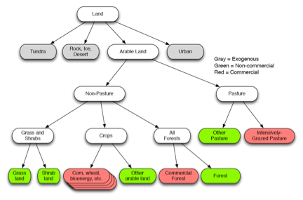
Figure 1: AgLU Land Nest

Intensification

The inclusion of multiple management types for each crop within each subregion of GCAM allows the model to represent price-induced intensification. That is, we can increase yields via increased fertilizer or irrigation if economic conditions favor those options. Like the rest of the land allocation decisions in GCAM, the share of each management practice depends on relative profitability. As profits of one option increase, more land will be allocated to that option. If the option is higher yielding, then average yields will increase (an intensification response). In general, GCAM will intensify when there is a lot of land competition (like when carbon in land is valued). Note that it is possible for average yields in a subregion to decline over time; this will happen if commodity prices decline or if the price of fertilizer and/or water increases.

Calibration

While the profit-based logit land sharing is fairly straightforward, it must be calibrated to match historical data on land use shares and profit rates in the base year. The calibration method solves for parameters that adjust observed profit rates, which are based on base year data, such that they equal the potential average profit rates implied by base year shares and the assumed average price of unmanaged land. In future model periods, the calibration profit scalers calculated in the final historical period are used to adjust the future profit rates in the logit sharing and profit equations. For more information, see the detailed description of the calibration. Additional information is also provided on modeling new land uses or crops and crop outliers.

Regional Production and Comparative Advantage

In its determination of the economic allocation of crop production and land use across regions of the globe, GCAM follows the basic economic principle of comparative advantage. In simplest terms, countries or regions will produce more of what they are better at and import more of what they are not as good at producing. For more information, see the detailed description of comparative advantage.

Terrestrial Carbon Approach

Land-use change CO₂ emissions are calculated in GCAM using a simple accounting approach, similar to that of Houghton (1999). That is, GCAM determines the change in above and below ground carbon stock for a given land use change and allocates that change in carbon stock over time.

Vegetation Carbon

For vegetation carbon, we distinguish between two different activities – land expansion and land contraction. In the event that land allocated to a particular type contracts, i.e., there is less land in the current period than the previous period, we assume that all vegetation carbon emissions are released instantaneously. In this event, the land-use change emissions for the current period from above ground carbon changes are equal to the change in above ground carbon stock. Emissions from above ground carbon changes for all other periods are equal to zero. In the event land expands, we spread the change in carbon stock across time depending on the length of time it takes for the vegetation to mature. For crops, the mature age is typically set a 1 year, meaning that all carbon uptake occurs instantaneously. For forests, however, we assume it takes anywhere from 30 years to 100 years to uptake all of the carbon. We use an example of the Bertalanffy-Richards function (see equation).

Soil Carbon

For soil carbon, we assume we assume both emissions and uptake are exponential, where the exponential half-life depends on the region. Colder regions have longer half-lives.

Carbon Stocks

GCAM tracks carbon stocks by calculating and storing cumulative land-use change emissions, and then applying those emissions as time proceeds. As land expands, we compute future uptake to be added to the carbon stock, and as land contracts we compute future emissions to subtract from the carbon stock.

Initialization of carbon density data for soil and vegetation carbon

The latest soil and vegetation carbon densities are initialized from inputs which are processed by the moirai land data system. moirai processes fine resolution soil carbon inputs from the Soilgrids dataset (Hengl et al. 2017) and similar vegetation carbon inputs from Spawn et al. (2020). These raw carbon densities represent the year 2010.

Soil carbon densities represent top soil (depth of 0-30 cm) and vegetation carbon densities are a sum of above and below ground biomass densities. As mentioned above, GCAM requires a steady state carbon density and not just the contemporary carbon density. The steady state carbon density is compatible with the GCAM methodology to represent land use transitions.

moirai thus calculates 6 “states” of carbon for each GLU land type combination when aggregating up the carbon densities from the gridcell level to the GLU land type level. The user can select any state of carbon by changing the constant aglu.CARBON_STATE in constants.R. The 6 states are, median_value (median of all available grid cells), min_value (minimum of all available grid cells), max_value (maximum of all available grid cells),weighted_average (weighted average of all available grid cells using the land area as a weight), q1_value (first quartile of all available grid cells) and q3_value (3rd quartile of all available grid cells).

The q3_value is the default for GCAM since it is the most representative of the steady state.

Note that the user can also change the data source for carbon densities itself to use the Houghton (1999) carbon densities by changing the parameter aglu.CARBON_DATA_SOURCE to “houghton” in constants.R.

Users interested in the moirai processing of the input data can refer to the detailed harmonization process described in the moirai Github repo.

Equations

The equations that determine land allocation and the resulting carbon emissions from land use and land cover change are described here.

Profit

Leaf profit

Profit for managed land leafs is calculated in the supply module and passed to the land allocator. Profit for unmanaged land leafs is input into the model. Within the land allocator, this profit is adjusted if land-related policies are included.

See setProfitRate in land_leaf.cpp and setUnmanagedLandProfitRate in unmanaged_land_leaf.cpp.

Node profit

The average profit of a node is calculated as

\[\pi_i = \left[{\sum_{j=1}^{N} \lambda_j^\rho \pi_j^\rho}\right]^{\frac{1}{\rho}}\]

where $\lambda_i$ is the profit scaler for leaf or node $i$, $\pi_i$ is the profit for node $i$, $\pi_j$ is the profit for leaf or node $j$ contained within node $i$, and $\rho$ is the logit exponent.

See calculateNodeProfitRates in land_node.cpp.

The share of each leaf or node is calculated as

\[s_i = \frac{(\lambda_i \pi_i)^\rho}{\sum_{j=1}^{N} (\lambda_j \pi_j)^\rho}\]

where $s_i$ is the share of leaf or node $i$, $\lambda_i$ is the profit scaler for leaf or node $i$, $\pi_i$ is the profit for leaf or node $i$, and $\rho$ is the logit exponent.

See calcLandShares in land_leaf.cpp and land_node.cpp.

Land Area

To calculate land area, GCAM works its way down the nesting tree, starting from the top where total land area in a region is provided as an input. For each node or leaf below, the area is calculated as

\[a_i = a_{above} * s_i\]

where $a_i$ is the area for leaf or node $i$, $s_i$ is the share, and $a_{above}$ is the area of the parent node.

See calcLandAllocation in land_leaf.cpp and land_node.cpp.

Calibration

To calibrate the land allocator, the share equation is inverted to solve for $\lambda_i$.

See calibrateLandAllocator in land_allocator.cpp and calculateShareWeights in land_node.cpp.

Carbon Emissions

The total cumulative change in emissions is calculated as

\[E^{veg/soil}_{t}=\Delta C_{t}=A_{t}*D^{veg/soil}_{t}-A_{t-1}*D^{veg/soil}_{t-1}\]

where $E$ indicates carbon emissions due to a land use change in timestep $t$, $C$ indicates carbon stocks, $A$ indicates land area, and $D$ indicates the average carbon density of the land area. These emissions are allocated over time differently for vegetation and soil carbon.

Vegetation Carbon Emissions

If vegetation emissions are positive (i.e., $E^{veg}_{t} > 0$), then all emissions are released in the current year, $y$. That is, $E^{veg}_{y} = E^{veg}_{t}$.

If vegetation emissions are negative, then these emissions are spread out over time using a sigmoid function:

\[E^{veg}_{y} = E^{veg}_{t} * \left[1 - e^{\frac{-3.0 * (y - t + 1)}{M}} \right]^2 - \left[1 - e^{\frac{-3.0 * (y - t)}{M}} \right]^2\]

where $t$ is the time of land conversion, $y$ is the current year, $M$ is the mature age (specified by land type and region).

See precalc_sigmoid_helper in land_carbon_densities.cpp for the implementation of the sigmoid and calcAboveGroundCarbonEmission in asimple_carbon_calc.cpp for the calculation of vegetation carbon emissions. For more information on the sigmoid function and its sensitivity to mature age, see Figure.

Soil Carbon Emissions

Soil carbon emissions follow an exponential approach:

\[E^{soil}_{y} = E^{soil}_{t} * \left[\left( 1.0 - e^{ -1.0 * \kappa * (y - t)} \right) - \left( 1.0 - e^{ -1.0 * \kappa * (y - t - 1)} \right)\right]\]

where $\kappa = \frac{ log(2) }{ s / 10.0}$ and $s$ is the soil time scale, specified by region (see inputs_land).

See calcBelowGroundCarbonEmission in asimple_carbon_calc.cpp for the calculation of soil carbon emissions.

Carbon Stock

Total carbon stock, $C_y$ in year $y$ is calculated as

\[C_y = C_{y-1} - \left[E^{veg}_{y-1} + E^{soil}_{y-1}\right]\]

where $E^{veg}_{y}$ are vegetation carbon emissions in year $y$ and $E^{soil}_{y}$ are soil carbon emissions in year $y$.

See calc in asimple_carbon_calc.cpp.

Policy options

This section summarizes some of the land-based policy options available in GCAM. More information on the trade-offs of these options is available in Calvin et al. (2014).

Protecting Lands

With this policy, we can set aside some land, removing it from economic competition. This will result in that land area being fixed across time and any land expansion/contraction will not affect this area.

(GCAM defualt) Protection constraints based on land suitability and protection constraints

By default, levels of available land for expansion are decided based on levels of suitability (as defined by Zabel et al. 2014) and protection constraints (as defined by the IUCN). There are 7 mutually exclusive types of land based on these suitability and protection constraints. They are:

Unsuitable and Unprotected
Suitable and Unprotected
Suitable with a high level of protection that is intact
Suitable with a high level of protection that is deforested
Suitable with a low level of protection
Unsuitable with a high value of protection
Unsuitable with a low value of protection.

By default land that is classified as Suitable and Unprotected (No 2 from the above) will be made available for expansion. The user can make other types of land available using the parameter aglu.NONPROTECT_LAND_STATUS in constants.R.

Specifying alternative percentage of available/protected land

The users can also set their own protection level, which is specified in the GCAM data system; see aglu.PROTECTION_DATA_SOURCE_DEFAULT in constants.R. Users can define a custom percentage of protected lands using the parameter aglu.PROTECT_DEFAULT.

Valuing Carbon in Land

In a policy regime, we can choose to put a price on land-use change CO₂ emissions that is related to the price on fossil fuel and industrial CO₂ emissions. The land carbon price can be any multiplier of the fossil fuel carbon price. This factor is applied at the geopolitical region level, and can be differentiated across regions. We model this policy as a subsidy to land-owners for the holding carbon stocks, as opposed to a tax/subsidy on the change in carbon in land. Specifically, the subsidy is equal to the carbon price x the carbon density x a discount factor to account for the amount of time it takes carbon to accumulate x a discount factor to annualize the subsidy.

An example file is included to implement this policy is included in GCAM; see global_uct.xml.

Bioenergy Constraints

We can impose constraints (lower or upper bounds) on bioenergy within GCAM. Under such a policy, GCAM will calculate the tax or subsidy required to ensure that the constraint is met. Note that by default a bioenergy constraint in GCAM (starting with v4.4) is imposed based on the amount of subsidy available for net negative emissions.

See Energy Constraint for an xml snippet.

Carbon densities

As mentioned above the user can also select different “states” of carbon other than the “q3_state” (which is considered the steady state). These include the weighted average, median, q1, min or max value. These can be selected in constant aglu.CARBON_STATE in constants.R.

Land expansion costs/constraints

One approach we have implemented and tested is to add a land expansion cost curve to targeted land types in specific regions. Specifically, we have added land expansion cost curves to unmanaged forest land in individual regions in which a carbon policy resulted in fast transformation from grassland to unmanaged forest. This method effectively adds a cost associated with converting to forests. This cost can be interpreted as the cost of planting, watering, fire management, etc. required to grow trees on previously unforested land.

The land expansion cost curve is implemented as a “renewable” resource that land must “purchase” on a per-unit of land basis. The cost curve can be set at a zero cost up to a predefined amount of land: e.g., base year allocation, pre-industrial allocation, etc. Beyond this point, the cost curve increases to either represent a physical expansion cost or an arbitrarily high cost that would act as a hard constraint on expansion. One drawback to this approach is that each cost curve adds a market equation that needs to be solved. The market should behave well, but adding markets should always be done with care as it does put additional burdens on the solution algorithm.

See Land Constraint for an xml snippet.

Carbon Parks

We have also included code to implement a crop technology that plants trees as densely as possible just for the purposes of storing carbon. Such a “carbon park” technology would allow us to explicitly include physical costs and demands for other inputs such as fertilizer and water when that modeling is available. This would clearly be a “managed” land option and would allow us some more options for modeling carbon policies. As with expansion costs/constraints, carbon parks are not a part of the current core configuration, but can be implemented through changes in input files.

Insights and intuition

Model evaluation

The GCAM land model has been evaluated using a hindcast experiment, as shown in Calvin et al. (2017) and Snyder et al. (2017). A few insights emerge from these studies. First, GCAM cannot predict policy, but the inclusion of policies that exist in the real world (e.g., biofuels targets) improves the performance of the model. Second, the use of forecasted yields to drive land allocation decisions improves the performance of the model as compared to using observed yields. Third, GCAM does better at trends than interannual variability. Finally, GCAM does better at some crops and regions than other crops and regions.

Sensitivity to parameters

The effect of a change in profitability of one land type on land allocation depends on the choice of parameters, as shown in Zhao et al. (2020). Larger logit exponents will result in a stronger transition to a land type whose profit increases than would occur with lower logit exponents. Note that this paper replicates the GCAM land allocation mechanism in a simple offline example and does not use the full GCAM.

Differences across regions

The effect of an increase in one type of land depends on where that increase occurs and what it displaces because of differences in regional land allocation and carbon densities as shown in Wise et al. (2015). For example, expanding bioenergy in a forested region will result in higher carbon emissions per unit of fuel produced than expanding bioenergy in a non-forested region.

Implications of policy

The choice of policy options in the land system has a dramatic effect on the resulting land allocation, resulting in changes in agricultural production, energy production, emissions, and prices. This result is demonstrated in Calvin et al. (2014). For example, policies that place a value on carbon in the land system will result in a transition to high carbon ecosystems (i.e., reforestation and afforestation). Policies that incentivize low carbon energy systems, without any additional incentives in the land system, result in large-scale deployment of bioenergy.

IAMC Reference Card

Land Cover

Agriculture and forestry demands

Agricultural commodities

Carbon dioxide removal

Bioenergy with CCS
Reforestation
Afforestation

References

Calvin, K., Wise, M., Kyle, P., Patel, P., Clarke, L., Edmonds, J., 2014. Trade-offs of different land and bioenergy policies on the path to achieving climate targets. Climatic Change 123, 691–704. https://doi.org/10.1007/s10584-013-0897-y.

Calvin, K., Wise, M., Kyle, P., Clarke, L., Edmonds, J., 2017. A hindcast experiment using the GCAM 3.0 agriculture and land-use module. Climate Change Economics 8. https://doi.org/10.1142/S2010007817500051

Hengl, T., Mendes de Jesus, J., Heuvelink, G. B., Ruiperez Gonzalez, M., Kilibarda, M., Blagotic, A., . & Guevara, M. A. (2017). SoilGrids250m: Global gridded soil information based on machine learning. PLoS one, 12(2), e0169748.

Houghton, R.A. 1999. The annual net flux of carbon to the atmosphere from changes in land use 1850-1990. Tellus 51B: 298-313.

Snyder, A. C., Link, R. P., & Calvin, K. V. (2017). Evaluation of integrated assessment model hindcast experiments: A case study of the GCAM 3.0 land use module. Geoscientific Model Development, 10(12). https://doi.org/10.5194/gmd-10-4307-2017.

Spawn, S.A., Sullivan, C.C., Lark, T.J. et al. Harmonized global maps of above and belowground biomass carbon density in the year 2010. Sci Data 7, 112 (2020)

Wise, Marshall, Calvin, Katherine, Page Kyle, Patrick Luckow, James Edmonds. 2014. Economic and Physical Modeling of Land Use in GCAM 3.0 and an Application to Agricultural Productivity, Land, and Terrestrial Carbon. Climate Change Economics. DOI 10.1142/S2010007814500031.

Wise, M., Hodson, E. L., Mignone, B. K., Clarke, L., Waldhoff, S., & Luckow, P. (2015). An approach to computing marginal land use change carbon intensities for bioenergy in policy applications. Energy Economics, 50, 337–347. https://doi.org/10.1016/j.eneco.2015.05.009

Zabel, Florian, Birgitta Putzenlechner, and Wolfram Mauser. “Global agricultural land resources-a high resolution suitability evaluation and its perspectives until 2100 under climate change conditions.” PloS one 9.9 (2014): e107522. https://doi.org/10.1371/journal.pone.0107522

Zhao, Xin, Katherine V. Calvin, and Marshall A. Wise. “The critical role of conversion cost and comparative advantage in modeling agricultural land use change.” Climate Change Economics 11, no. 01 (2020): 2050004. https://doi.org/10.1142/S2010007820500049

Name	Resolution	Unit	Source
Historical land use and land cover	By GLU, land type, and year	thousand \(km^2\)	Exogenous
Vegetation carbon density	By GLU and land type	kg per \(m^2\)	Exogenous
Soil carbon density	By GLU and land type	kg per \(m^2\)	Exogenous
Mature age	By GLU and land type	years	Exogenous
Soil time scale	By geopolitical region and land type	years	Exogenous
Value of unmanaged land	By GLU	1975$ per thous \(km^2\)	Exogenous
Profit rate of managed land	By GLU	1975$ per thous \(km^2\)	Land Supply Module
Logit exponents	By GLU and land node	Unitless	Exogenous

The GCAM Land Allocation Module

Table of Contents

Inputs to the Module

Description

Economic Modeling Approach

Land Sharing Approach

Land Nesting Strategy

Intensification

Calibration

Regional Production and Comparative Advantage

Terrestrial Carbon Approach

Vegetation Carbon

Soil Carbon

Carbon Stocks

Initialization of carbon density data for soil and vegetation carbon

Equations

Profit

Leaf profit

Node profit

Shares

Land Area

Calibration

Carbon Emissions

Vegetation Carbon Emissions

Soil Carbon Emissions

Carbon Stock

Policy options

Protecting Lands

(GCAM defualt) Protection constraints based on land suitability and protection constraints

Specifying alternative percentage of available/protected land

Valuing Carbon in Land

Bioenergy Constraints

Carbon densities

Land expansion costs/constraints

Carbon Parks

Insights and intuition

Model evaluation

Sensitivity to parameters

Differences across regions

Implications of policy

IAMC Reference Card

References