Quickstarter#
The purpose of this tutorial is to demonstrate how stitches can be
used as an emulator. While stitches can emulate a number of CMIP6
models this example will focus on emulating CanESM5 SSP245 results.
To use stitches, there are a number of decisions users have to make,
perhaps the most important being:
Which ESM will
stitchesemulate?What archive data will be used? These are values that the target data will be matched to. It should only contain data for the specific ESM that is being emulated. Users may limit the number of experiments or ensemble realizations within the archive in order to achieve their specific experimental setup.
What target data will be used? This data frame represents the temperature pathway the stitched product will follow. The contents of this data frame may come from CMIP6 ESM results for an SSP or it may follow some arbitrary pathway.
A diagram illustrating the stitches process is included for
reference:
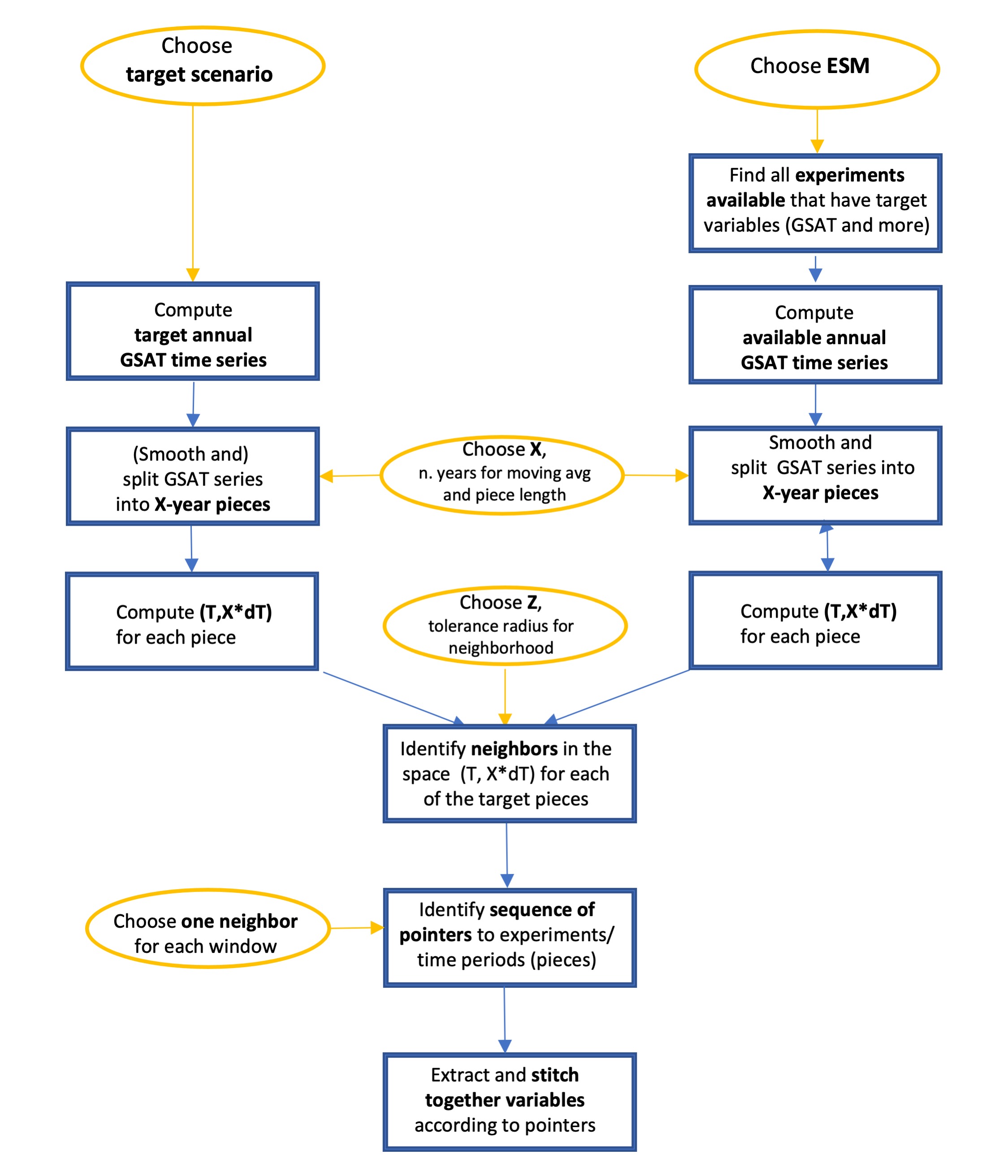
stitches workflow#
stitchesdefaults to \(X=9\) year windows.
Getting Started#
Start by loading the stitches package (see installation
instructions if stitches is
not yet installed).
import stitches
Load the additional python libraries that will be used in this example.
These packages are installed as stitches dependencies.
import os
import pkg_resources
import warnings

import numpy as np
import pandas as pd
from matplotlib import pyplot as plt


# For help with plotting
%matplotlib inline
%config InlineBackend.figure_format = 'retina'
plt.rcParams['figure.figsize'] = 12, 6
Install the package data from Zenodo#
The package data is all data that has been processed from raw Pangeo data and is generated with package functions. For convenience and rapid cloning of the github repository, the package data is also minted on Zenodo and can be quickly downloaded for using the package.
stitches.install_package_data()
Example 1: Emulate global mean air temperature#
We will begin with an example focused on emulating global mean air temperature before moving on to an example producing gridded data for multiple variables.
The global mean air temperature (GSAT) is the key variable upon which
stitches operates to construct new realizations, with the added
benefit that it is easy to visualize.
Example Set Up#
In this example, we will use stitches to emulate CanESM5 SSP245
results. Then we will compare the stitches results with actual CMIP6
CanESM5 SSP245 output data.
Decide on the archive data#
Limit the archive matching data to the model we are trying to emulate, CanESM5 in this case.
In this example, we treat SSP245 as a novel scenario rather than one run by the ESM and available, so we exclude it from the archive data.
The internal package data called
matching_archivecontains the temperature results for all the ESMs-Scenarios-ensemble members that are available forstitchesto use in its matching process. In this file monthly, tas output has been processed to mean temperature anomaly and the temperature change over a window of time. By defaultstitchesuses a 9-year window.
# read in the package data of all ESMs-Scenarios-ensemble members avail.
data_directory = pkg_resources.resource_filename('stitches', "data")
path = os.path.join(data_directory, 'matching_archive.csv')
data = pd.read_csv(path)

archive_data = data.loc[(data["experiment"].isin(['ssp126',  'ssp370', 'ssp585']))
                       & (data["model"] == "CanESM5")].copy()
Modify Inputs - Decide on the target data#
The primary input to
stitchesfunctions that most users will adjust is the target data.The target data is the temperature pathway the stitched (emulated) product will follow. This data can come from an ESM or another class of climate models, for a specific SSP scenario or an arbitrarily defined scenario. Similarly to the archive data, the target data should contain the mean temperature anomaly and rate of temperature change over a window of time. The target data window and the archive window must be the same length,
stitchesuses a 9-year window by default.In this example because we are demonstrating
stitchesability to emulate CanESM5 SSP245, we will use CanESM5 SSP245 results for a single ensemble member to use as our target data.
# Load time series and subset to target time series if needed:
targ = pd.read_csv(os.path.join(data_directory, "tas-data", "CanESM5_tas.csv"))
target_data = targ.loc[(targ["model"] == "CanESM5")
                       & (targ["experiment"] == 'ssp245')].copy()

target_data  = target_data[target_data["ensemble"].isin(['r1i1p1f1'])].copy()

target_data = target_data.drop(columns='zstore').reset_index(drop=True)
Take a look at the structure and a plot of the time series we will be targeting:
print(target_data.head())
target_data.plot(x='year', y='value')
plt.show()
plt.close()
  variable experiment  ensemble    model  year     value
0      tas     ssp245  r1i1p1f1  CanESM5  1850 -1.133884
1      tas     ssp245  r1i1p1f1  CanESM5  1851 -1.389375
2      tas     ssp245  r1i1p1f1  CanESM5  1852 -1.318175
3      tas     ssp245  r1i1p1f1  CanESM5  1853 -1.163771
4      tas     ssp245  r1i1p1f1  CanESM5  1854 -1.302066
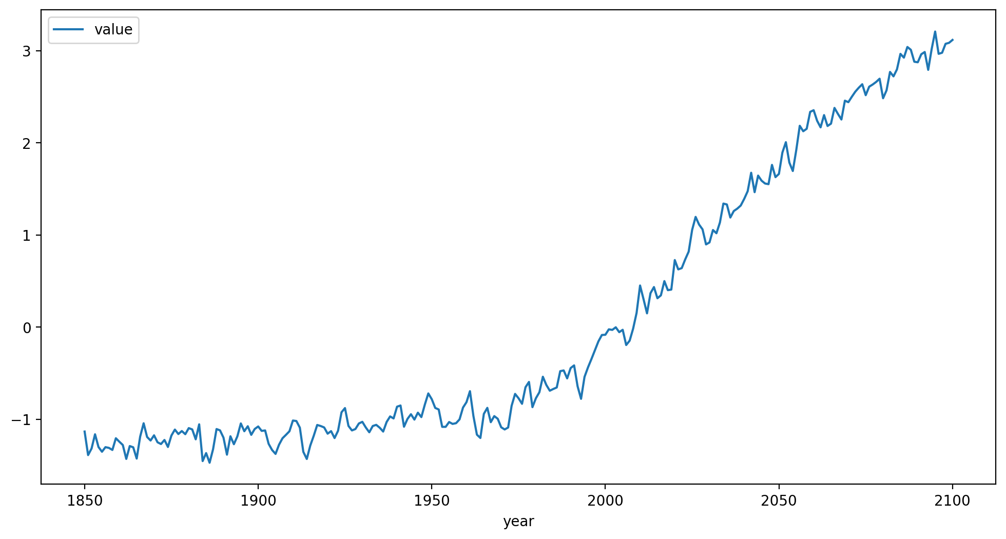
Any time series of global average temperature anomalies can be used as a target. However, the data frame containing this time series must be structured as above: a
variablecolumn containing entries of ‘tas’,yearandvaluecolumns containing the data, andexperiment,ensemble,modelcolumns with identifying information of the source of this target data.The actual entries in the
experiment,ensemble,modelcolumns are only used for generating identifying strings for generated ensemble members.In this demonstration, we will specifically be targeting ensemble member 1 of the CanESM5 SSP245 simulations. The entire SSP245 ensemble may be jointly targeted by omitting the line
target_data = target_data[target_data["ensemble"].isin(['r1i1p1f1'])].copy()
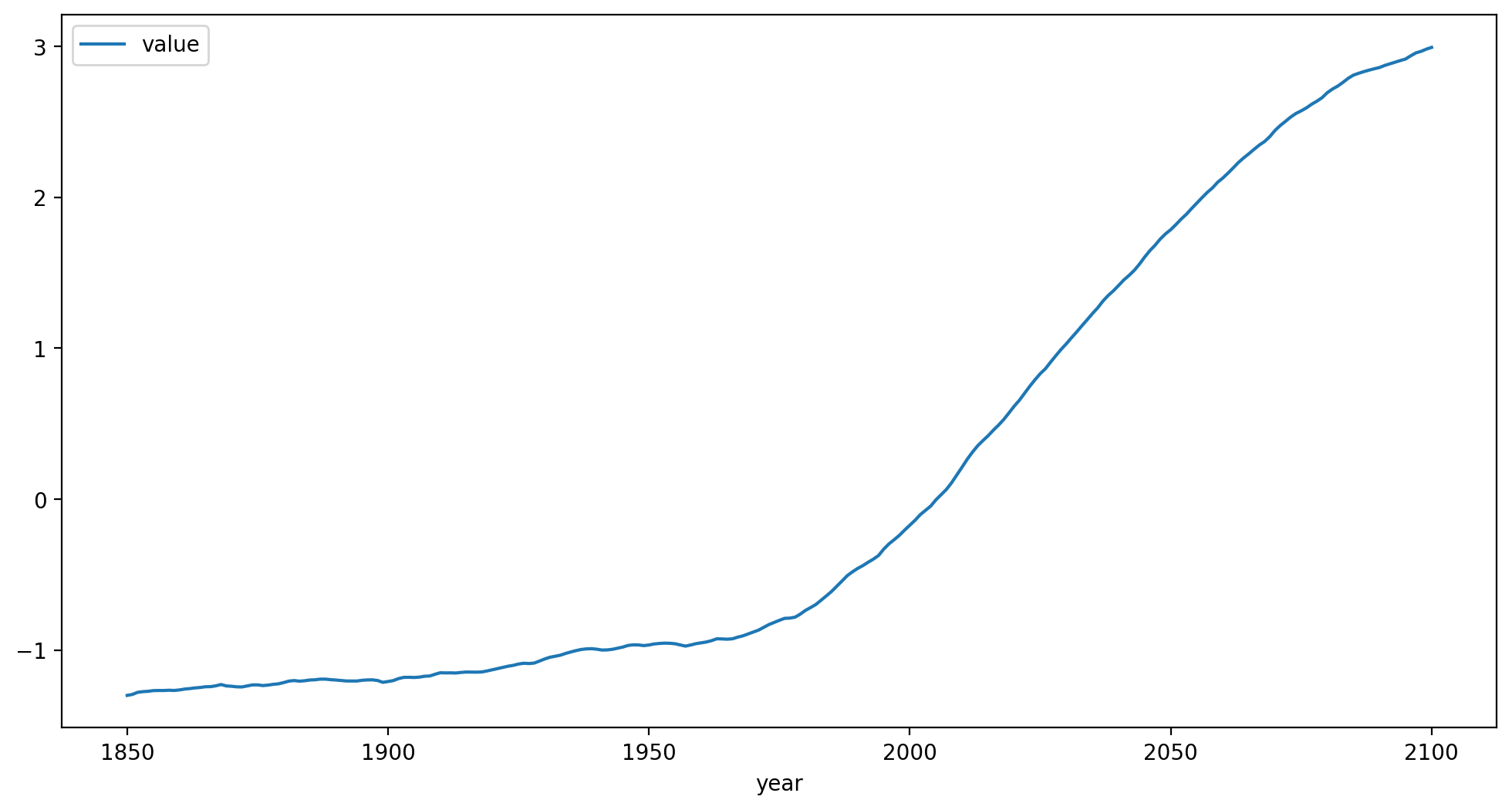
Modify Inputs - Prepare target data for matching#
stitches includes functions that convert the above data frame of raw
target data into correctly structured target data for matching.
# First, smooth the target data
target_data = stitches.fx_processing.calculate_rolling_mean(target_data,
                                                            size=31).copy()
target_data.plot(x='year', y='value')
plt.show()
plt.close()

# then process so it can be matched on:
target_data = stitches.fx_processing.get_chunk_info(
    stitches.fx_processing.chunk_ts(df = target_data,  n=9)).copy()
Use the target_data and archive_data to make the recipes using the function make_recipe()#
We ask for 4 new realizations to be constructed, and we specify that the matching be limited to a
tol(\(Z\) in the diagram) value of 0.06degC.tolis the parameter that effectively controls both the maximum number of generated time series that may be constructed and the quality of matches.For large values of
tol, the matches constructed may be no good. Currently, the cutoff values oftolfor each ESM are determined by post-hoc calculation, as described in the ESD paper.we use the
reproducibleargument so that the results are reproducible. It is not required and can be set toFalseto have a random draw of generated recipes
my_recipes = stitches.make_recipe(target_data,
                                  archive_data,
                                  tol=0.06,
                                  N_matches=4,
                                  reproducible=True)
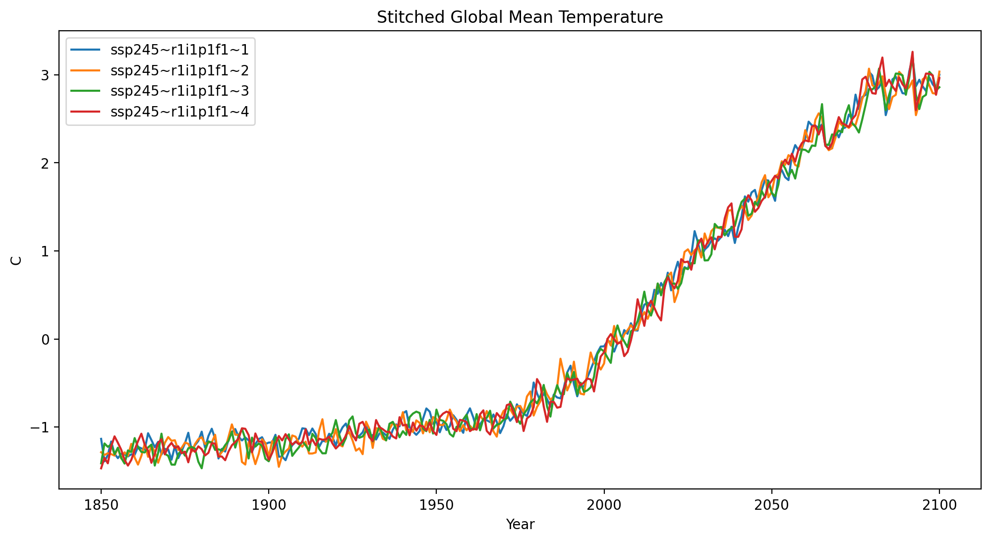
Now use the recipe to get the global mean air temperature using
gmat_stitching. The data frame returned by gmat_stitching will
contain the final stitched product.
stitched_global_temp = stitches.gmat_stitching(my_recipes)
Visualize Results#
groups = stitched_global_temp.groupby('stitching_id')

for name, group in groups:
    plt.plot(group.year, group.value, label = name)

plt.xlabel("Year")
plt.ylabel("C")
plt.title("Stitched Global Mean Temperature")
plt.legend()
plt.show()
plt.close()
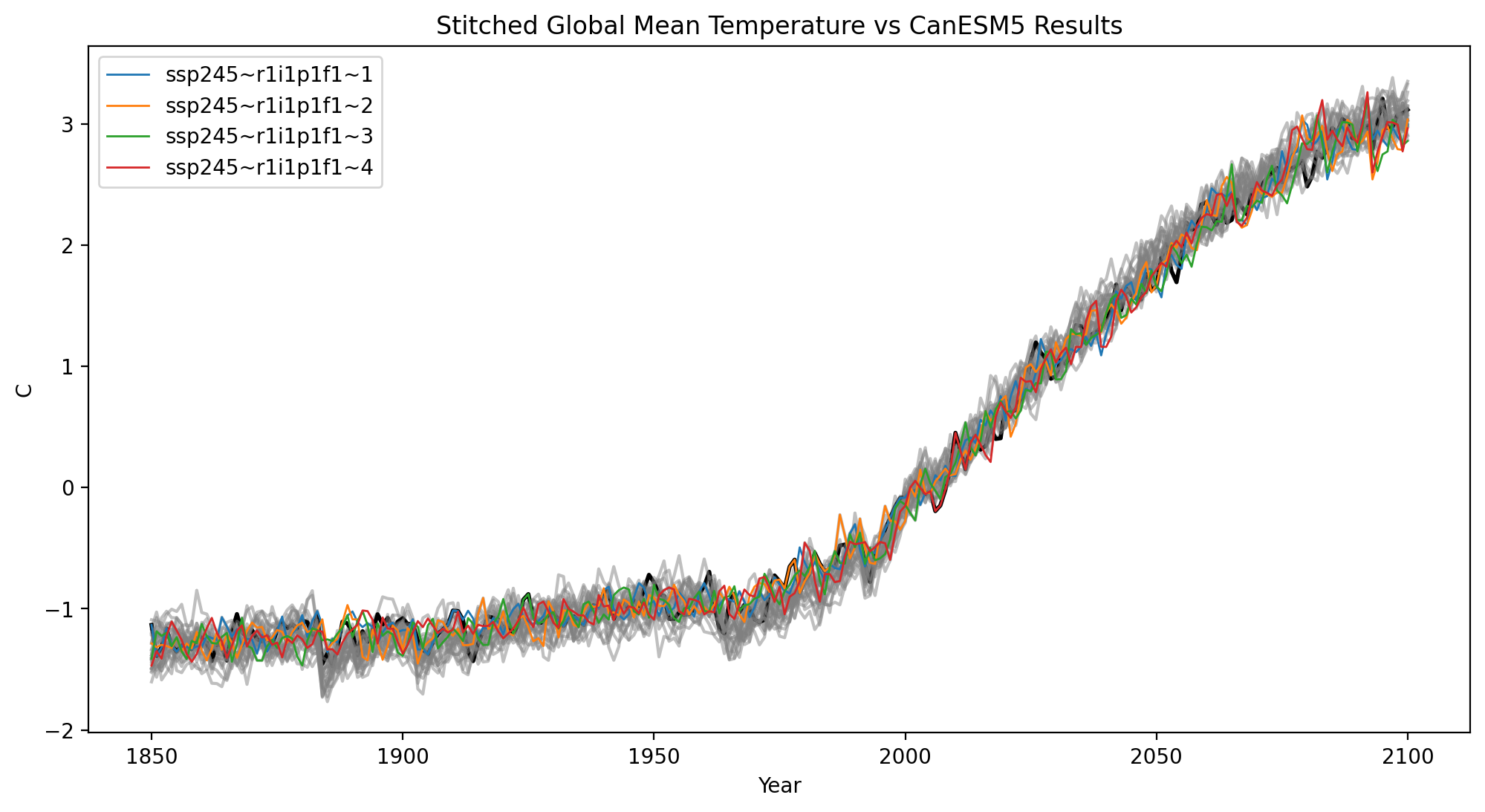
Now let’s compare the stitched products with the actual CanESM5 SSP245 data#
The black curve is realization 1 - the ESM data that this notebook actually targeted.
The gray curves are the other archived realizations of SSP245 for CanESM5 to illustrate that the generated ensemble members do not systematically depart from the actual ensemble behavior.
GSAT data is included as package data in
stitchesfor convenience.
# Load the comparison GSAT data
data_path = pkg_resources.resource_filename('stitches', 'data/tas-data/CanESM5_tas.csv')

comp_data = pd.read_csv(data_path)
comp_data = comp_data.loc[comp_data["experiment"] == "ssp245"]
# full ensemble of actual ESM runs:
groups = comp_data.groupby('ensemble')
for name, group in groups:
    if(group.ensemble.unique() == 'r1i1p1f1'):
        plt.plot(group.year, group.value, color = "black", linewidth = 2.0)
    else:
        plt.plot(group.year, group.value, color = "0.5", alpha=0.5)

# The stitched realizations:
groups = stitched_global_temp.groupby('stitching_id')
for name, group in groups:
    plt.plot(group.year, group.value, linewidth= 1.0, label = name)

plt.legend()
plt.xlabel("Year")
plt.ylabel("C")
plt.title("Stitched Global Mean Temperature vs CanESM5 Results")
plt.show()
plt.close()
Example 2: stitching gridded products for multiple variables.#
With the basis of matching illustrated in the example 1, we highlight
especially the structure of the “recipes” stitches creates:
print(my_recipes.iloc[0,])
target_start_yr                                                    1850
target_end_yr                                                      1858
archive_experiment                                           historical
archive_variable                                                    tas
archive_model                                                   CanESM5
archive_ensemble                                               r1i1p1f1
stitching_id                                          ssp245~r1i1p1f1~1
archive_start_yr                                                   1850
archive_end_yr                                                     1858
tas_file              gs://cmip6/CMIP6/CMIP/CCCma/CanESM5/historical...
Name: 0, dtype: object
The tas_file entry points to the specific CMIP6 netcdf file on
pangeo that must be pulled for these years to create a gridded
temperature product. To create a recipe that can produce a gridded
product for multiple variables we will need to use
stitches.make_recipe() with the argument non_tas_variables set
to the additional variables of interest.
Match and stitch#
As in example 1 set up the target and archive data. We will be using the same setup for CanESM5 ssp245.
Set the
non_tas_variables= “pr” to indicate that the recipe should include precipitation results (seehelp(stitches.make_recipe)for more details onnon_tas_variables). Now the resulting recipe includestas_fileandpr_filecolumns that point to CMIP6 files fortasandprmonthly data on pangeo. These files will be pulled from pangeo and data for these years will be used to create the gridded data product.Variables other than surface air temperature and precipitation may be considered.
In this example we will only generate a recipe for one new realization for expediency, but
N_matchesmay be increased with no changes to the stitching calls below.
my_recipes = stitches.make_recipe(target_data,
                                  archive_data,
                                  tol=0.06,
                                  non_tas_variables=['pr'],
                                  N_matches=1,
                                  reproducible=True)
To stitch new realizations of the gridded data as netcdfs, use the
function gridded_stitching. The results are saved in a
user-specified directory. In this example, it is the same directory this
notebook sits in.
These netcdf files may then be read in and examined with xarray
functions.
For speed, this block is not executed by default in the quickstart. Instead, we have pre-built and uploaded these netcdfs for easy exploration.
stitches.gridded_stitching(out_dir='.', rp=my_recipes)
Load generated data#
# load the stitched (generated) temperature (tas) netcdf files
gen_tas = stitches.fetch_quickstarter_data(variable="tas")

# load the stitched pr netcdf file
gen_pr = stitches.fetch_quickstarter_data(variable="pr")
Fetch target data from pangeo for comparison#
# Fetch the actual data directly from pangeo
pangeo_path = pkg_resources.resource_filename('stitches', 'data/pangeo_table.csv')

pangeo_data = pd.read_csv(pangeo_path)

pangeo_data = pangeo_data.loc[(pangeo_data['variable'].isin(['tas', 'pr']))
                              & (pangeo_data['domain'].str.contains('mon'))
                              & (pangeo_data['experiment'].isin(['ssp245']))
                              & (pangeo_data['ensemble'].isin(['r1i1p1f1']))
                              & (pangeo_data['model'].isin(['CanESM5']))].copy()

pangeo_data
| model | experiment | ensemble | variable | zstore | domain | |
|---|---|---|---|---|---|---|
| 21843 | CanESM5 | ssp245 | r1i1p1f1 | pr | gs://cmip6/CMIP6/ScenarioMIP/CCCma/CanESM5/ssp... | Amon |
| 21910 | CanESM5 | ssp245 | r1i1p1f1 | tas | gs://cmip6/CMIP6/ScenarioMIP/CCCma/CanESM5/ssp... | Amon |
# load the target tas netcdf files
tas_address = pangeo_data.loc[pangeo_data['variable']== 'tas'].zstore.copy()
tar_tas = stitches.fetch_nc(tas_address.values[0])

# load the target pr netcdf files
pr_address = pangeo_data.loc[pangeo_data['variable']== 'pr'].zstore.copy()
tar_pr = stitches.fetch_nc(pr_address.values[0])
Visualize#
Select a grid cell and plot the generated and target tas, pr data for first-cut comparison
def plot_comparison(generated_data,
                    target_data,
                    variable,
                    alpha=0.8):
    """Plot comparision between target variable time series and generated data"""

    if variable.casefold() == "pr":
        variable_name = "precipitation"
        units = "kg m-2 s-1"
    else:
        variable_name = "temperature"
        units = "C"

    # temperature (tas)
    plt.plot(generated_data.time,
             generated_data[variable],
             label=f"Generated monthly {variable}")

    with warnings.catch_warnings():
        warnings.filterwarnings("ignore")

        plt.plot(target_data.indexes['time'].to_datetimeindex(),
                 target_data[variable],
                 alpha=alpha,
                 label = f"Target monthly {variable}")

    plt.legend()
    plt.xlabel("Year")
    plt.ylabel(units)
    plt.title(f"Actual and generated monthly {variable_name} ({variable})")
    plt.show()
    plt.close()
# lon and lat values for a grid cell near the Joint Global Change Research Institute in College Park, MD, USA
cp_lat = 38.9897
cp_lon = 180 + 76.9378

# lat and lon coordinates closest
abslat = np.abs(gen_tas.lat - cp_lat)
abslon = np.abs(gen_tas.lon-cp_lon)
c = np.maximum(abslon, abslat)
([lon_loc], [lat_loc]) = np.where(c == np.min(c))
lon_grid = gen_tas.lon[lon_loc]
lat_grid = gen_tas.lat[lat_loc]

cp_tas_gen = gen_tas.sel(lon=lon_grid,
                         lat=lat_grid,
                         time=slice('2015-01-01', '2099-12-31')).copy()

cp_tas_tar = tar_tas.sel(lon=lon_grid,
                         lat=lat_grid,
                         time=slice('2015-01-01', '2099-12-31')).copy()

cp_pr_gen = gen_pr.sel(lon=lon_grid,
                       lat=lat_grid,
                       time=slice('2015-01-01', '2099-12-31')).copy()

cp_pr_tar = tar_pr.sel(lon=lon_grid,
                       lat=lat_grid,
                       time=slice('2015-01-01', '2099-12-31')).copy()

# temperature (tas)
plot_comparison(generated_data=cp_tas_gen,
                target_data=cp_tas_tar,
                variable="tas")

# precipitation (pr)
plot_comparison(generated_data=cp_pr_gen,
                target_data=cp_pr_tar,
                variable="pr")
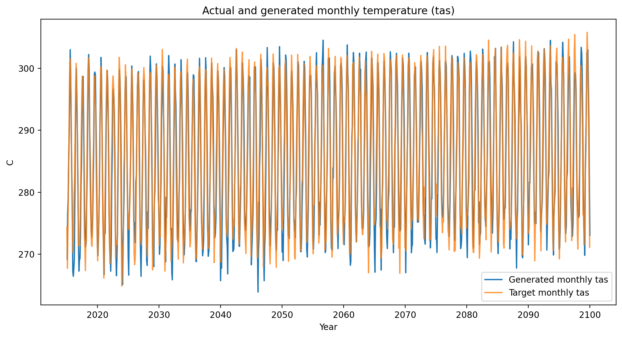
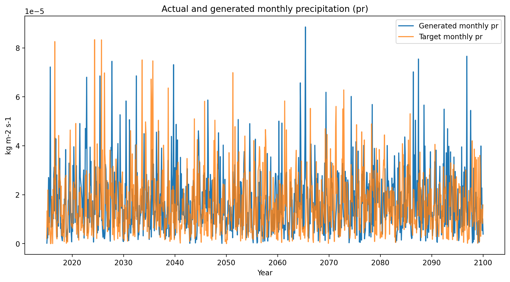
Visual validation of the complex spatial, temporal, and cross-variable relationships present in ESM outputs is not possible. We extensively validate that the method reproduces ESM internal variability in the ESD paper, but this visual plotting at least suggests that nothing is obviously wrong.
In other words, it’s not inconceivable from these plots that the orange time series were sampled from the same underlying multivariate distribution that generated the blue time series.