GCAM v5.1 Documentation: GCAM Shared-Socioeconomic Pathways
Documentation for GCAM
The Global Change Analysis Model
View the Project on GitHub JGCRI/gcam-doc
GCAM Shared-Socioeconomic Pathways
Overview of the SSPs
The GCAM model was one of six models used in the quantification of the Shared Socioeconomic Pathways (SSP; Riahi et al., 2017). The SSPs are new reference scenarios for climate change modeling and research (Moss et al. 2010, van Vuuren et al., 2014). That is the five SSPs assume no additional policies and measures explicitly designed to reduce greenhouse gas emissions. However, each of the five reference scenarios can be paired with a set of emissions mitigation assumptions. Thus, when paired with a limit of 2.6, 4.5, or 6.0, the resulting scenario can be used in combination with the corresponding climate model experiments in the CMIP data base. The five SSPs are defined along two different axes: challenges to mitigation and challenges to adaptation (see Figure below).
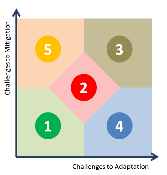
Figure 1: Definitions of SSPs in terms of Challenges to Mitigation and Challenges to Adaptation
Each of the six IAMs produced results for between three and five of the SSPs, with one model identified as the “marker” for each SSP and the others providing estimates of uncertainty. GCAM was the marker model for the SSP4. Marker models, and models providing uncertainty estimates, for all SSPs are listed in the Table below.
Table 1: Overview of the SSPs
| Identifier | Descriptor | Marker Model (Institution) | Also computed by |
|---|---|---|---|
| SSP1 | Sustainability | IMAGE (PBL) | All |
| SSP2 | Middle-of-the-Road | MESSAGE-GLOBIOM (IIASA) | All |
| SSP3 | Regional Rivalry | AIM/CGE (NIES) | GCAM, IMAGE, MESSAGE-GLOBIOM |
| SSP4 | Inequality | GCAM (PNNL) | AIM/CGE |
| SSP5 | Fossil-fueled Development | REMIND-MAgPIE (PIK) | AIM/CGE, GCAM |
Accessing SSP Data
Official SSP data, as planned for use in CMIP6, must be downloaded from the official SSP database.
The GCAM data for the SSP4 and the GCAM representation of all other SSPs (Calvin et al., 2017) are being made available to interested researchers for scenario analysis and comparison.
Implementation in GCAM
To implement the SSPs within GCAM, we use the demographic and economic assumptions developed by Lutz et al. (2015) and Dellink et al. (2015) in combination with technology and policy assumptions derived from the SSP narratives (O’Neill et al. 2015). Table 2 provides a qualitative summary of these parameters; quantitative details are provided in subsequent tables. In general, we have altered parameters related to energy supply (e.g., the capital cost of new power plants, technical change on extraction costs), energy demand (e.g., preferences for traditional bioenergy), agriculture (e.g., agricultural productivity growth), and policy (e.g., start years for carbon policies). To implement the SSP storylines within GCAM, we quantified “high”, “medium”, and “low” for each of the variables listed in Table 2. Those quantifications are provided in Table 3 through Table 8.
Table 2: Qualitative Assumptions across SSPs
| Category | Variable | SSP1 | SSP2 | SSP3 | SSP4 (High / Medium / Low Income ) | SSP5 |
|---|---|---|---|---|---|---|
| Socioeconomics | Population in 2100 | 6.9 billion | 9 billion | 12.7 billion | 0.9 billion / 2.0 billion / 6.4 billion | 7.4 billion |
| GDP per capita in 2100 | $46,306 | $33,307 | $12,092 | $123,244 / $30,937 / $7,388 | $83,496 | |
| Fossil Resources (Technological Change/Acceptance) | Coal | Med/Low | Med/Med | High/High | Med/Low / Med/Med / Med/High | High/High |
| Conventional Gas & Oil | Med/Med | Med/Med | Med/Med | High/Low / High/Low / High/Low | High/High | |
| Unconventional Oil | Low/Med | Med/Med | Med/Med | Med/Low / Med/Low / Med/Low | High/High | |
| Electricity (Technology Cost) | Nuclear | High | Med | High | Low /Low / Low | Med |
| Renewables | Low | Med | High | Low / Low / Low | Med | |
| CCS | High | Med | Med | Low / Low / Low | Low | |
| Fuel Preference | Renewables | High | Med | Med | High / High / High | Med |
| Traditional Biomass | Low | Low | High | Low / Low / High | Low | |
| Energy Demand (Service Demands) | Buildings | Low | Med | Low | High / Med / Low | High |
| Transportation | Low | Med | Low | High / Med / Low | High | |
| Industry | Low | Med | Low | High / Med / Low | High | |
| Agriculture & Land Use | Food Demand | High | Med | Low | High / Med / Low | High |
| Meat Demand | Low | Med | High | Med / Med / Med | High | |
| Productivity Growth | High | Med | Low | High / Med / Low | High | |
| Trade | Global | Global | Global | Regional / Regional / Local | Global | |
| SPA* Policy | Afforestation | Limited afforestation | No land policy | Afforestation / Limited afforestation / No land policy | Afforestation | |
| Pollutant Emissions | Emissions Factors | Low | Med | High | High / High / High | Low |
| Marker | Model | IMAGE | MESSAGE-GLOBIOM | AIM | GCAM | REMIND-MAGPIE |
| Reference | Van Vuuren et al. (2016) | Riahi et al. (2016) | Fujimori et al. (2016) | Calvin et al. (2016) | Kriegler et al. (2016) | |
| Challenges | Challenges to Mitigation | Low | Medium | High | Low | High |
| Challenges to Adaptation | Low | Medium | High | High | Low |
Electricity Assumptions
Table 3 maps technology & SSP to either core, advanced (less expensive), or low (more expensive). Costs are assumed to be equal across regions; however, resource bases for renewable energy technologies differ across regions, leading to differences in deployment in the future.
Table 3: Capital Costs for Electric Power Plants across SSPs
Plant Type |
SSP1 |
SSP2 |
SSP3 |
SSP4 |
SSP5 |
Nuclear |
LOW |
CORE |
LOW |
ADV |
CORE |
Geothermal |
ADV |
CORE |
LOW |
ADV |
CORE |
PV |
ADV |
CORE |
LOW |
ADV |
CORE |
PV with storage |
ADV |
CORE |
LOW |
ADV |
CORE
|
Rooftop PV |
ADV |
CORE |
LOW |
ADV |
CORE |
CSP |
ADV |
CORE |
LOW |
ADV |
CORE |
CSP with storage |
ADV |
CORE |
LOW |
ADV |
CORE |
Wind |
ADV |
CORE |
LOW |
ADV |
CORE |
Wind with storage |
ADV |
CORE |
LOW |
ADV |
CORE |
Fossil Fuel Assumptions
Table 4 details assumptions made for fossil fuel supply. Similar to renewables, we do not vary the resource bases across SSPs, but instead vary cost of extraction and use. In particular, we adjust the technical change coefficient on future extraction costs to reflect differences in technological conditions across SSPs. To reflect differences in social acceptance, we use a cost adder that adjusts the cost to downstream users. The cost adder for 2100 is shown in Table 3; adders are linearly interpolated from $0 in 2010 to the 2100 value. The 2100 value is defined in relation to the carbon content of the resource; thus, a “medium” social acceptance will result in a different cost adder for different fuels.
Table 4a: Fossil Fuel Assumptions across SSPs: Technical Change on Extraction Cost (% per year)
| Fuel | SSP1 | SSP2 | SSP3 | SSP4 | SSP5 |
|---|---|---|---|---|---|
| Coal | 0.5% | 0.5% | 1% | 0.5% | 2% |
| Gas | 0.5% | 0.5% | 0.5% | 1% | 2% |
| Conventional Oil | 0.5% | 0.5% | 0.5% | 1% | 2% |
| Unconventional Oil | 0% | 0.5% | 0.5% | 2% |
Table 4b: Fossil Fuel Assumptions across SSPs: Cost Adder in 2100 ($/GJ)
| Fuel | SSP1 | SSP2 | SSP3 | SSP4 | SSP5 |
|---|---|---|---|---|---|
| Coal | $1.37 | $0.27 | $0 | $0.27 | $0 |
| Gas | $0.14 | $0.14 | $0.14 | $0.71 | $0 |
| Conventional Oil | $0.20 | $0.20 | $0.20 | $0.98 | $0 |
| Unconventional Oil | $0.21 | $0.21 | $0.21 | $1.06 | $0 |
Building Energy Demand Assumptions
Table 5 includes information on implementation of the SSPs for building energy demand. In particular we adjust the rate at which traditional bioenergy is phased out across SSPs. This is done in GCAM by adjusting the fuel preference elasticity, a parameter that links preferences (i.e., the share weight of the logit function) to per capita income. More negative fuel preference elasticities result in faster phase outs. This parameter is used to capture differences in intraregional inequality between SSP3 and SSP4; namely, we assume a faster phase out for the same income level in SSP3 than in SSP4.
Table 5: Building energy demand Assumptions
|
SSP1 |
SSP2 |
SSP3 |
SSP4 |
SSP5 |
Fuel Preference Elasticity for Traditional Bioenergy |
-2.5 |
-2 |
-1 |
-0.75 |
-2.5 |
Agriculture and Land Use Assumptions
Table 6 includes information on implementation of the SSPs for the agriculture and land-use sector. For agricultural productivity growth, we relate the parameters used in each SSP to the GCAM default assumptions. These assumptions are based on FAO projections through 2050, then held constant at 0.25%/yr post-2050. The projections in the near-term vary by crop, region, management practice (irrigated vs. rainfed), and year. As a result, there are literally thousands of parameters in a single scenario. For ease of presentation, we describe our assumptions for the individual SSPs with respect to the GCAM default. For food demand, all SSPs assume that growth in food demand is linked to income, using historical income-calorie relationships. To capture differences in food preferences and food waste, we adjust meat consumption and preferences in different SSPs. Finally, trade restrictions on agriculture and bioenergy are imposed in the SSP3 and SSP4.
Table 6: Agriculture and Land Use Assumptions across SSPs
| Variable | SSP1 | SSP2 | SSP3 | SSP4 (High / Med / Low Income ) | SSP5 |
|---|---|---|---|---|---|
| Agricultural Productivity Growth | 50% above GCAM default | GCAM default | 50% below GCAM default | 50% above GCAM default / GCAM default / 50% below GCAM default | 50% above GCAM default |
| Meat Demand | Meat demand limited to 1000 kcal/per/day. Shift in preferences among meat products away from beef, sheep, and goats. | Meat demand limited to 1100 kcal/per/day. | Meat demand limited to 1400 kcal/per/day. | Meat demand limited to 1100kcal/per/day. | Meat demand limited to 1400 kcal/per/day. |
Climate Policy
To move from baseline scenarios to the RCP replications, we implemented the Shared Policy Assumptions (Kriegler et al., 2014) in GCAM. These assumptions are described in Table 7. For land policy, the relevant policy is phased in over several decades once the globally harmonized carbon price is imposed. For CO2 prices prior to global cooperation, we impose the carbon price required to reach a region’s Copenhagen pledge in an SSP2 world in all SSPs. That is, the same carbon price in 2020 is used regardless of SSP. Note that these policy assumptions are not unique and alternative assumptions could be derived that are also consistent with the SSP storylines. Note that the land carbon price described in the table is absent any transaction costs; we further reduce carbon prices on land by 50% to capture these effects.
Table 7a: Policy Assumptions across SSPs: First model time period with global cooperation (i.e., harmonized global carbon price)
| Income Group | SSP1 | SSP2 | SSP3 | SSP4 | SSP5 |
|---|---|---|---|---|---|
| High Income | 2025 | 2040 | 2040 | 2025 | 2040 |
| Medium Income | 2025 | 2040 | 2040 | 2025 | 2040 |
| Low Income | 2025 | 2040 | 2050 | 2025 | 2040 |
Table 7b: Policy Assumptions across SSPs: Land Policy
| Income Group | SSP1 | SSP2 | SSP3 | SSP4 | SSP5 |
|---|---|---|---|---|---|
| High Income | Carbon Price on Land is Equal to Energy Carbon Price (i.e., UCT in Wise et al., 2009) | Carbon Price on Land is Equal to 50% of Energy Carbon Price | No Land Policy (i.e., FFICT in Wise et al., 2009) | Carbon Price on Land is Equal to Energy Carbon Price (i.e., UCT in Wise et al., 2009) | Carbon Price on Land is Equal to Energy Carbon Price (i.e., UCT in Wise et al., 2009) |
| Medium Income | Carbon Price on Land is Equal to Energy Carbon Price (i.e., UCT in Wise et al., 2009) | Carbon Price on Land is Equal to 50% of Energy Carbon Price | No Land Policy (i.e., FFICT in Wise et al., 2009) | Carbon Price on Land is Equal to 50% of Energy Carbon Price | Carbon Price on Land is Equal to Energy Carbon Price (i.e., UCT in Wise et al., 2009) |
| Low Income | Carbon Price on Land is Equal to Energy Carbon Price (i.e., UCT in Wise et al., 2009) | Carbon Price on Land is Equal to 50% of Energy Carbon Price | No Land Policy (i.e., FFICT in Wise et al., 2009) | No Land Policy (i.e., FFICT in Wise et al., 2009) | Carbon Price on Land is Equal to Energy Carbon Price (i.e., UCT in Wise et al., 2009) |
Differences between Official SSPs and GCAM5.1 SSPs
The official SSPs (Calvin et al., 2017) were branched from GCAM4.0. There are several changes between versions that will have implications for SSP-related results. First, in the original SSPs (Calvin et al., 2017), electricity power plant costs were based off of the values used in GCAM4.0. We defined advanced and low as deviations from the core model. GCAM4.2, however, updated the power plant capital costs in the core, and established advanced and low technology costs. These values will be used going forward in the SSPs. Second, GCAM5.1 includes different land regions and multiple land technologies (see below). These are likely to have effects on all land-related results. Third, GCAM4.4 introduced a net negative emissions constraint that wasn’t present in the official SSPs. This will affect bioenergy use and net negative CO2 emissions, particularly in 2.6 W/m2 scenarios.
Data from the official SSPs is available at SSP database.
References
Calvin, K., B. Bond-Lamberty, L. Clarke, J. Edmonds, J. Eom, C. Hartin, S. Kim, P. Kyle, R. Link, R. Moss, H. McJeon, P. Patel, S. Smith, S. Waldhoff and M. Wise (2017). “The SSP4: A world of deepening inequality.” Global Environmental Change 42: 284-296.
Dellink, R., et al., Long-term economic growth projections in the Shared Socioeconomic Pathways. Global Environ. Change (2016), http://dx.doi.org/10.1016/j.gloenvcha.2015.06.004
Kriegler, E., Edmonds, J., Hallegatte, S., Ebi, K. L., Kram, T., Riahi, K., Winkler, H. & Van Vuuren, D. P. 2014. A new scenario framework for climate change research: The concept of shared climate policy assumptions. Climatic Change, 122, 401-414.
Lutz, KC, S., W., The human core of the shared socioeconomic pathways: Population scenarios by age, sex and level of education for all countries to 2100. Global Environ. Change (2016), http://dx.doi.org/10.1016/j.gloenvcha.2014.06.004
Moss, R. H., J. A. Edmonds, K. A. Hibbard, M. R. Manning, S. K. Rose, D. P. van Vuuren, T. R. Carter, S. Emori, M. Kainuma, T. Kram, G. A. Meehl, J. F. B. Mitchell, N. Nakicenovic, K. Riahi, S. J. Smith, R. J. Stouffer, A. M. Thomson, J. P. Weyant and T. J. Wilbanks (2010). “The next generation of scenarios for climate change research and assessment.” Nature 463(7282): 747-756.
O’Neill, Brian C., Elmar Kriegler, Kristie L. Ebi, Eric Kemp-Benedict, Keywan Riahi, Dale S. Rothman, Bas J. van Ruijven et al. “The roads ahead: Narratives for shared socioeconomic pathways describing world futures in the 21st century.” Global Environmental Change (2016). doi:10.1016/j.gloenvcha.2015.01.00
Riahi, K., D. P. van Vuuren, E. Kriegler, J. Edmonds, B. C. O’Neill, S. Fujimori, N. Bauer, K. Calvin, R. Dellink, O. Fricko, W. Lutz, A. Popp, J. C. Cuaresma, S. Kc, M. Leimbach, L. Jiang, T. Kram, S. Rao, J. Emmerling, K. Ebi, T. Hasegawa, P. Havlik, F. Humpenöder, L. A. Da Silva, S. Smith, E. Stehfest, V. Bosetti, J. Eom, D. Gernaat, T. Masui, J. Rogelj, J. Strefler, L. Drouet, V. Krey, G. Luderer, M. Harmsen, K. Takahashi, L. Baumstark, J. C. Doelman, M. Kainuma, Z. Klimont, G. Marangoni, H. Lotze-Campen, M. Obersteiner, A. Tabeau and M. Tavoni (2017). “The Shared Socioeconomic Pathways and their energy, land use, and greenhouse gas emissions implications: An overview.” Global Environmental Change 42: 153-168.
van Vuuren, D. P., E. Kriegler, B. C. O’Neill, K. L. Ebi, K. Riahi, T. R. Carter, J. Edmonds, S. Hallegatte, T. Kram, R. Mathur and H. Winkler (2014). “A new scenario framework for Climate Change Research: scenario matrix architecture.” Climatic Change 122(3): 373-386.