GCAM v5.1 Documentation: GCAM Emissions
Documentation for GCAM
The Global Change Analysis Model
View the Project on GitHub JGCRI/gcam-doc
GCAM Emissions
Overview
GCAM projects emissions of a suite of greenhouse gases (GHGs) and air pollutants:
CO2, CH4, N2O, CF4, C2F6, SF6, HFC23, HFC32, HFC43-10mee, HFC125, HFC134a, HFC143a, HFC152a, HFC227ea, HFC236fa, HFC245fa, HFC365mfc, SO2, BC, OC, CO, VOCs, NOx, NH3
Future emissions are determined by the evolution of drivers (such as energy consumption, land-use, and population) and technology mix. How this is represented in GCAM varies by emission type.
Table Of Contents
- CO2 Emissions
- CO2 Emissions From Land-Use/Land-Use Change (LULUC)
- Non-CO2 Emissions Overview
- Non-CO2 GHG Emissions
- Air Pollutant Emissions
- Advanced Non-CO2 User Options
CO2 Emissions
GCAM endogenously estimates CO2 fossil-fuel related emissions based on fossil fuel consumption and global emission factors by fuel (oil, unconventional oil, natural gas, and coal). These emission factors are consistent with global emissions by fuel from the CDIAC global inventory (CDIAC 2017).
GCAM can be considered as a process model for CO2 emissions and reductions. CO2 emissions change over time as fuel consumption in GCAM endogenously changes. Application of Carbon Capture and Storage (CCS) is explicitly considered as separate technological options for a number of processes, such as electricity generation and fertilizer manufacturing. The GCAM, in effect, produces a Marginal Abatement Curve for CO2 as a carbon-price is applied within the model.
CO2 emissions from limestone used in cement production are also estimated. Limestone consumption has one global emissions factor, however, each region’s IO coefficient (limestone / cement) is calibrated to return CDIAC estimates (CDIAC 2017). (CO2 from fuel consumed in producing limestone is estimated in the same manner as other fuel consumption.)
CO2 emissions from gas flaring are not currently included in GCAM.
CO2 Emissions From Land-Use/Land-Use Change (LULUC)
Land-Use Change emissions are tracked separately. In general, emissions are estimated as:
\[E_{r,t}=\Delta S_{r,t}=A_{r,t}*C_{r,t}-A_{r,t-1}*C_{r,t-1}\]Where E indicates carbon emissions, S indicates carbon stocks, A indicates land area, and C indicates the average carbon density of the land area, across all land use types.
When land is converted to forests, the vegetation carbon content of that new forest land exponentially approaches an exogenously-specified, region-dependent value in order to represent the finite time required for forests to grow, as shown in the figure below.
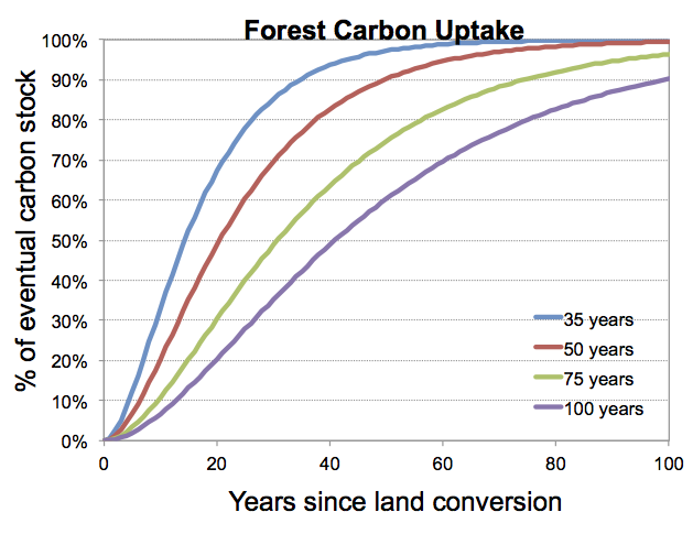
Figure 1: Timescales for forest regrowth in GCAM.
Changes in the carbon content of soils due to land-use change also exponentially approach an equilibrium value using a region-dependent timescale. This represents the timescales for carbon pool changes in soils.
Non-CO2 Emissions Overview
We summarize here some general points common to non-CO2 emissions in GCAM
Non-CO2 emissions, both GHGs & air pollutants, originate from many sources and can be controlled using multiple abatement technologies. Modeling non-CO2 abatement at the process level would require too much detail for the scales at which GCAM operates. We, therefore, use parameterized functions for future emissions controls (for air pollutants) and Marginal Abatement Cost (MAC) curves (for GHGs) to change emission factors over time. The emissions controls, which reduce emissions factors as a function of per-capita GDP in each region and time period, are based on the general understanding that pollutant control technologies are deployed as incomes rise (e.g., Smith et al. 2005, although the functional form used in GCAM 5 is different than that in this reference). The MAC curves for GHGs are mapped directly to GCAM’s technologies from the EPA’s 2013 report on non-CO2 greenhouse gas mitigation (EPA 2013).
Note that technology shifts still play a role, since emission factors can differ between technologies.
Most base-year non-CO2 emissions are calibrated to the EDGAR 4.2 emissions inventories (EDGAR 2011), with USA fuel-level emissions detail from the US EPA’s National Emissions Inventory (EPA 2011) used to disaggregate sectoral totals to specific fuel types. Black carbon (BC) and organic carbon (OC) emissions are calibrated using the RCP (CMIP5) inventories (Lamarque et al. 2010). Additional information on fluorinated gases is from Guus Velders.
Energy System Drivers
- Emissions in the energy system can be driven by input (e.g., fuel consumed by a particular technology) or output (e.g., fuel or service produced by a particular technology).
- Emissions information is technology-specific. As a result, different technologies that produce the same output can have different emissions per unit of activity.
- For most gases and species, we explicitly model the drivers for the emissions. However, for some (e.g., HFCs from fire extinguishers), the future emissions scale directly with population and/or GDP.
Agriculture and Land-Use Drivers
- Emissions in the agriculture and land use system can be driven by output (e.g., for crop production) or land area (e.g., for forest fires).
- Emissions are modeled at the level of agricultural technologies: region, water basin, crop type, and irrigation and management level. Note however that the underlying inventory data is far coarser, typically only available by sector and country.
Naming Conventions
There are some naming conventions for a few emission species/sectors within GCAM that are useful to note.
- Emissions from most agricultural activities are suffixed with “_AGR”, except for burning of agricultural waste on fields (AWB), which are suffixed with “_AWB”. (This allows us to separate emissions from these distinct processes from the same technology.) These are in addition to emissions named without a suffix. So to obtain total emissions, the three variants of a given species should be added (e.g., CH4 emissions is the sum of CH4, CH4”_AGR”, and CH4”_AWB”.)
- Sulfur dioxide (SO2) emissions are currently differentiated by four metaregions (SO2_1,SO2_2,SO2_3,SO2_4). These are kept separate for purposes of feeding the emissions information to the climate model; for emissions estimation, these different categories should be added to obtain global totals.
Non-CO2 GHG Emissions
The non-CO2 greenhouse gases include methane (CH4), nitrous oxide (N2O) and fluorinated gases. These emissions, E, are modeled for any given technology in time period t as:
\[E_{t}=A_{t}*F_{t0}*(1-MAC(Cprice_{t})))\]where:
| F | Emissions factor: base-year emissions per unit activity |
| A | Activity level (e.g., output of a technology) |
| MAC | Marginal Abatement Cost Curve |
| Eprice | Emissions Price |
Non-CO2 GHG emissions are proportional to the activity except for any reductions in emission intensity due to the MAC curve. As noted above, the MAC curves are assigned to a wide variety of technologies, mapped directly from EPA 2013. Under a carbon policy, emissions are reduced by an amount determined by the MAC curve.
The default set-up is that MAC curves use the scenario’s carbon price (if any). The non-CO2 GHG MACs are an exogenous input, and are read in as the percent of emissions abated as a function of the emissions prices. Note that they are read in with explicit cost points (i.e., piece-wise linear form), with no underlying equation describing the percentage of abatement as a function of the carbon price.
Below-zero (i.e. “no cost”) MAC mitigation (e.g. MAC reduction percentage is > 0 at zero carbon price) are applied in the reference case and phased in over several decades. (This can be turned off by setting the no-zero-cost-reductions option to 1 within a MAC curve.)
Note that a species-specific emissions market can also be specified using advanced options, described below.
Fluorinated Gases
Most fluorinated gas emissions are linked either to the industrial sector as a whole (e.g., semiconductor-related F-gas emissions are driven by growth in the “industry” sector), or population and GDP (e.g., fire extinguishers). As those drivers change, emissions will change. Additionally, we include abatement options based on EPA MAC curves.
SF6 emissions from electric transformers scale with electricity consumption. HFC134a from cooling (e.g., air conditioners) scale with air conditioner electricity consumption. For these emissions we also make additional exogenous adjustments to emissions factors in future periods in developing regions to reflect their continued transition from CFCs to HFCs.
Air Pollutant Emissions
Air pollutant emissions such as sulfur dioxide (SOs) and nitrogen oxides (NOx) are modeled as:
\[E_{t}=A_{t}*EF_{t0}*(1-EmCtrl(pcGDP_{t}))\]where EmCtrl is a function that represents decreasing emissions intensity as per-capita income increases:
\[EmCtrl_{t}=1-\frac{1}{1+\frac{(pcGDP_{t}-pcGDP_{t0})}{steepness}}\]where pcGDP stands for the per-capita GDP, and steepness is an exogenous constant, specific to each technology and pollutant species, that governs the degree to which changes in per-capita GDP will be translated to emissions controls. The purpose here is to capture the general global trend of increasing pollutant controls over time, but does not capture regional and technological heterogeneity.
Note that the GCAM implementation of the SSP scenarios used a different approach, incorporating region-, sector-, and fuel-specific pollutant emission factor pathways (Calvin et al. 2017, Rao et al. 2017).
Advanced Non-CO2 User Options
Markets
For information on using markets for non-CO2 emissions see the markets For non-CO2 section of the polices page.
Additional Non-CO2 Emission Options
Emission objects can be added/changed via user input in any time period. New parameters (such as emission factors) overwrite any previous values. Note that emission control objects will be copied forward. For vintaged technologies (e.g. electric generation, road transport), any new emission object will be applied to new vintages. Old vintages will retain the previously read-in emission characteristics.
This also means that GHG objects can be removed or overwritten after a given year by reading in a new GHG object for that gas. This also applies to GHG control objects. Reading in a new control object, for example, in 2020 for an electric generation technology will negate the effect of a previously read in control object of the same name for that vintage and future vintages. This can, for example, represent a transition from some emissions control regime applied to older vintages to a regime defined by new source performance standards.
In addition to the GDP control object, a linear-control object is also available that allows a user to specify that an emission factor will linearly change over time to a user-defined value over a specified time period. The parameters controlling the linear-control object are:
| XML Tag | Description |
|---|---|
| end-year | Year by which emission factor should reach specified value |
| start-year | (Optional) Start year after which EF should begin to decline. (defaults to final calibration year) |
| final-emissions-coefficient | Emissions coefficient that should be set by end-year (and every year thereafter) |
| allow-ef-increase | (optional) Allow emission factors to increase from their start-year value (default to false) |
References
[Calvin et al. 2017] Calvin, K., Bond-Lamberty, B., Clarke, L., et al. 2017. The SSP4: a world of deepening inequality. Global Environmental Change 42: 284–296. doi:10.1016/j.gloenvcha.2016.06.010. Link
[CDIAC 2017] Boden, T., and Andres, B. 2017, National CO2 Emissions from Fossil-Fuel Burning, Cement Manufacture, and Gas Flaring: 1751-2014, Carbon Dioxide Information Analysis Center, Oak Ridge National Laboratory. Link
[EDGAR 2011] Joint Research Centre. 2011. EDGAR - Emissions Database for Global Atmospheric Research: Global Emissions EDGAR v4.2. doi:10.2904/EDGARv4.2. Link
[EPA 2011] US EPA, 2011, 2011 National Emissions Inventory (NEI) Data. United States Environmental Protection Agency, Office of Air Quality Planning and Standards. Link
[EPA 2013] US EPA, 2013, Global Mitigation of Non-CO2 Greenhouse Gases: 2010-2030. EPA-430-R-13-011, United States Environmental Protection Agency, Office of Atmospheric Programs. Link
[Lamarque et al. 2010] Lamarque, J.F., Bond, T. C., Eyring, V., et al. 2010. Historical (1850-2000) gridded anthropogenic and biomass burning emissions of reactive gases and aerosols: methodology and application, Atmospheric Chemistry and Physics 10(15): 7017–7039. doi:10.5194/acp-10-7017-2010. Link
[Rao et al. 2017] Rao, S., Klimont, Z., Smith, S., et al. 2017. Future air pollution int he Shared Socio-economic Pathways. Global Environmental Change 42: 246–358. doi:10.1016/j.gloenvcha.2016.05.012. Link
[Smith et al. 2005] Smith, S.J., Pitcher, H., and Wigley, T. 2005. “Future Sulfur Dioxide Emissions” Climatic Change 3: 267-318. doi: 10.1007/s10584-005-6887-y. Link