GCAM v4.4 Documentation: GCAM-USA
Documentation for GCAM
The Global Change Analysis Model
View the Project on GitHub JGCRI/gcam-doc
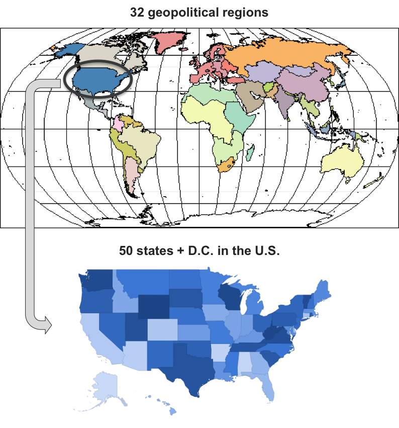
GCAM-USA
The Global Change Assessment Model (GCAM) and GCAM-USA
The GCAM model was expanded to include greater spatial detail in the USA region, referred to as GCAM-USA. In GCAM-USA the 50 U.S. states plus the District of Columbia (hereafter, the 51 states) are included as explicit regions that operate within the global GCAM model. Energy transformation (electricity generation and refined liquids production) and end-use demands (buildings, transportation, and industry) are modeled at the individual state level. Inter-state trade of all energy goods is considered, with state-specific consumer price mark-ups assigned for coal, natural gas, and refined liquids assigned based on price data from EIA (2012).
Note, several aspects of the energy system are still modeled at the aggregate U.S. level. Most notably this applies to primary production of fossil resources including oil, gas, and coal. The supply of biomass energy feedstocks, which include residues and dedicated energy crops, is modeled at the level of 10 agro-ecological zones (AEZ) in the United States (Calvin et al 2014, Wise et al 2014). As with primary fossil resources, biomass feedstocks are assumed to be freely traded at one global price.
Developing a historical energy balance for model calibration
The first step to modeling at the 51 state level was to create energy balances–that is, production and consumption of different forms of energy by each modeled sector, fuel, and state. This data was developed from 1971 to the final historical year of 2010, and applied in the model base years of 1975, 1990, 2005, and 2010. While more recent data are available, in order to incorporate the more recent historical data in the GCAM-USA module, the entire global energy and agricultural balances in GCAM, as well as land cover by land use type, would all need to be updated. Similarly, in the data processing of the state-level energy data, the aggregated national GCAM-USA energy balances (i.e., all states added together) must still be equal to the corresponding flows in the USA region of the global GCAM data set, which are derived from International Energy Agency (IEA) Energy Balances. With this in mind, we use portional allocations to disaggregate the US-level quantity flows to the states, utilizing state level data sets from the US Energy Information Agency (EIA). The EIA SEDS (State Energy Data System) was used as the primary data set for this purpose (EIA 2014a). The main steps of the data processing methods are described in the subsequent sections.
End-use sectors
We begin by describing the process for developing the energy balances for final energy demands including the buildings, transportation, and industry sectors. Compared with energy transformation sectors, these are relatively simple because (as modeled) their outputs are considered final demands, not commodities traded across states (as opposed to energy transformation sectors whose outputs and inputs must be considered).
Additional processing to differentiate energy for specific buildings services required additional data sets and assumptions as described in Zhou et al. (2013). Each of up to 10 modeled energy services (e.g., space heating, space cooling, water heating, etc.) can be supplied by one or more technologies. Heating and cooling service demand depends on building envelope thermal efficiency, internal heat gains, and climate. Technology and building envelope efficiencies are assumed to increase over the century as described in Zhou et al (2014).
As in the remainder of GCAM, the transportation sector in GCAM-USA is disaggregated to three final demands: passenger, domestic freight, and international shipping. The demand for each of these transportation services (indicated in passenger-km or tonne-km) depends on the base-year service demand levels, and the future growth in GDP and population by state. Each of the freight and passenger vehicle classes represent on-road vehicle options such as cars, trucks, and motorcycles, as well as off-road options such as trains, airplanes, and/or ships. For road modes, specific vehicle options include various size classes and drivetrain technologies differentiated by fuel type and/or efficiency levels, such as liquid fuels, hybrid drivetrains, and battery electric propulsion. These assumptions are consistent with the transporation sector in the global GCAM model: Energy System. The following mapping from the EIA SEDS is used in order to assign nation-level energy consumption and service demand levels by mode and fuel to the individual states.
Table: EIA SEDS fuel and sector used to disaggregate nation-level energy consumption by mode and fuel to the states.
| Mode | GCAM fuel | EIA fuel used for disaggregation |
|---|---|---|
| Air Domestic | refined liquids | Jet fuel in transporation |
| Air International | refined liquids | Jet fuel in transporation |
| Bus | gas | Natural gas in vehicle fuel |
| Bus | refined liquids | Distillate fuel oil in transporation |
| HSR | electricity | Electricity in transporation |
| LDV_2W | electricity | Electricity in transporation |
| LDV_2W | refined liquids | Motor gasoline in transportation |
| LDV_4W | electricity | Electricity in transporation |
| LDV_4W | gas | Motor gasoline in transportation |
| LDV_4W | hydrogen | Motor gasoline in transportation |
| LDV_4W | refined liquids | Motor gasoline in transportation |
| Rail | coal | Distillate fuel oil in transporation |
| Rail | electricity | Electricity in transporation |
| Rail | refined liquids | Distillate fuel oil in transporation |
| Ship Domestic | refined liquids | Residual fuel oil in transportation |
| Ship International | refined liquids | Residual fuel oil in transportation |
| Truck | refined liquids | Distillate fuel oil in transporation |
| Truck | gas | Distillate fuel oil in transporation |
Industrial energy allocations require more complicated processing steps, due to the refinery sector’s energy use being included in the industry sector of SEDS, as well as the need to assign nation-level electricity co-generation at industrial facilities. The national estimates of cogeneration by fuel are from the IEA’s Autoproducer CHP Plants, defined as facilities whose power production is primarily in support of activities that are on-site. No state-and fuel-level inventory of co-generation was available, so fuel consumption by the whole industrial sector is used to derive the state-wise portional allocations of both the fuel inputs and electricity outputs to/from cogeneration.
As in the remainder of the model, cement and N fertilizer are modeled specifically by state, with the state-wise allocation of energy consumption and physical outputs based on the value of shipments of the corresponding NAICS code. Specifically, cement is disaggregated by the value of shipments from 3273: Cement and concrete product manufacturing. Fertilizer is disaggregated by 3253: Pesticide, fertilizer, and other agricultural chemical mfg. States with zero output from these industries in the historical years are assumed to remain that way in future years as well.
Refining sector
In the EIA’s state-level data, refinery energy use is tracked under the industrial sector, with nothing to distinguish it from the remainder of the sector except that it is the only part of the industrial sector that consumes raw crude oil, which is a fuel commodity in SEDS. The amount of crude oil consumed by the industrial sector in the EIA database is therefore used as the basis for disaggregation of the national estimates for inputs and outputs of crude oil refining. We assume the same refinery input-output coefficients in all states (i.e., the same amounts of gas, electricity, and crude oil consumed per unit of refined liquids produced); therefore, given the amount of crude oil consumed as energy by the industrial sector (i.e., petroleum refineries) in each state, we can calculate the amount of electricity and gas consumed, and the amount of refined liquid products produced. The calculated amounts of gas and electricity that are inputs to refineries in each state are then deducted from the balance of the industrial sector’s energy consumption.
For biomass liquids, the energy output (biofuel production) for the whole USA is disaggregated among states according to each state’s share of production, using EIA (2014b) for biodiesel, and the SEDS inventory for ethanol production, which is estimated to scale with reported “biofuels energy losses and co-products.” Note that the biofuel feedstocks (corn kernels, soybean oil) are considered as agricultural commodities (i.e., not as energy commodities), and as such are not modeled at the state level in GCAM-USA. The only EIA fuels considered as biomass are wood and waste, neither of which are modeled as feedstocks for liquid biofuels in the historical calibration years. However, the biofuel production processes are modeled as consumers of natural gas and electricity; these quantities are calculated from the state-level production volumes using exogenous input-output coefficients, and deducted from the balance of the industrial sector.
Liquid fuels used as industrial feedstocks for the whole nation are then disaggregated to states on the basis of the sum of asphalt and petrochemical feedstocks consumption in each state. Natural gas used as feedstocks (i.e., used for non-energy purposes) is not explicitly accounted in the EIA SEDS database. This is not surprising as (a) unlike liquid fuels, there is nothing different about the natural gas used as feedstocks from that used for energy, and (b) the characterization of gas as “feedstock” as opposed to “energy” is a difficult one which is only done post-hoc based on product yields, and only in some energy inventories. Moreover, in many cases (e.g. ammonia production, hydrogen production), even the “feedstock” uses of natural gas entail 100% release of fuel carbon as CO2. In any case, the IEA-based national estimate of natural gas feedstocks is disaggregated to states on the basis of each state’s share of the whole nation’s use of (liquid fuel) petrochemical feedstocks, which are used as a proxy for the size of the chemicals industry in each state. This amount of gas is then deducted from the SEDS estimate of industrial energy use of gas in each state. Note also that most of the natural gas “feedstocks” in the US (estimated in the IEA Energy Balances) are for ammonia production; see IEA (2009) for a description of the accounting methods. Because ammonia production is explicitly modeled, this national estimate of natural gas feedstocks in GCAM is considerably lower than the number in the IEA Energy Balances.
Electric sector
Next we will describe creating the 51 state energy balance for the electric sector, starting with electricity generation. The EIA SEDS database represents hydrocarbon-fueled electricity only by fuel inputs to the electricity sector (EI in the SEDS database), with all other technologies represented only in terms of electricity output (EG). State-level thermal-electric efficiency is therefore not determinable from the data. As such, we apply the national average electric generation efficiency by fuel (calculated from the IEA energy balance data) to all states.
At this stage we have estimated total electricity generation from central production as well as CHP by state. Together these constitute the input to the GCAM “electricity net ownuse” sector, equal to total net generation, including electricity consumed on-site. The next step is to subtract each state’s own use of electricity. Own use of electricity is disaggregated to states on the basis of the “Direct Use” by states in the EIA, 2008b, Table A1: Selected Electric Industry Summary Statistics by State, 2008. As with all other sectors, the GCAM USA region’s total for electricity ownuse is disaggregated to states according to each state’s share in the table cited above. By subtracting own use, we then have the output of the electricity_net_ownuse sector in each state, which is the net input into the electricity transmission and distribution grid.
Finally we estimate electricity losses with in each state. EIA SEDS presents estimates of energy losses in transmission and distribution. The method for calculating the coefficient for electricity is to first add up all of the demands of electricity by all sectors: refining, electricity, buildings, industry, and transportation. Then the electricity T&D energy losses are added in, with the total of all the state estimates scaled to match the IEA’s whole-US estimates of electricity distribution losses.
A number of assumptions regarding technology characteristics in the electric power sector need to be made. Generally speaking assumptions are carried from the USA region of GCAM and applied equally to all states. This includes generation efficiencies, costs, and technology availability. Regional variations in resource characteristics such as wind and solar potential and geothermal and carbon storage resources are accounted for.
Electricity Trade
For electricity trade between states we group states roughly into the 13 NEMS Electricity Market Module Regions (EIA 2010) plus Alaska and Hawaii. Whereby states within the same sub-region can trade freely within that sub-region, trade between regions may be limited.
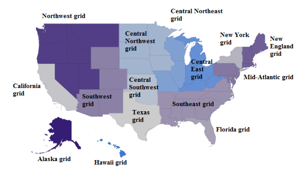
Modeled electricity markets based on NEMS.
Renewable Energy
Renewable energy resources are modeled at the state level. Wind and residential rooftop PV technologies include a separation between state-specific resource cost curves, which represent marginal costs that increase with deployment, plus technology capital costs that are the same in all states, but whose costs are levelized in the model with state-specific capacity factors. The escalation of the supply curve reflects factors such as transmission line costs that would be required to produce power from remote wind resources, and reducing capacity factors as the most optimal locations are used first. Central station solar technologies are assumed to have constant marginal costs regardless of deployment levels, but with state-specific capacity factors. Wind resource curves are based on Zhou, et al. 13. Geothermal resources are from Lopez A, et al. 14. Supply curves for residential rooftop PV are obtained from Denholm and Margolis 15. Hydro power is held fixed at historical production levels.
Carbon-Dioxide Capture and Geologic Storage
The depiction of the grid-region-specific graded CO2 transport storage cost curves reflect adjusted per-ton project costs for CO2 transport and geologic storage as based on the methodology developed by Dahowski et al. (2011); Dahowski et al. (2005); Dahowski et al. (2010). The costs shown in the figure include site characterization, capital and operations and maintenance costs associated with CO2 injection into suitable deep geologic reservoirs, and costs for required measurement, monitoring and verification technologies as well as other costs associated with regulatory compliance. These values do not include the cost of CO2 capture and compression to pipeline pressures, which are accounted for at the level of the technologies of emissions-producing activities that are equipped to perform CO2 capture. CO2 storage is aggregated to the same sub-regional markets as electricity to allow for some cross state border trade in CO2.
The region-specific CO2 transport and storage cost curves for the U.S. were developed using a cost-optimized source-sink matching algorithm designed to model globally optimal CCS deployment (again, less the cost of CO2 capture and compression) across the modeled domain. Each point on the resulting cost curves represents a single source-sink pair with a single average per-ton cost over the first 20-year timestep of the analysis (see Dahowski et al., 2005; Dahowski et al., 2010 for the rationale for this 20-year time step and its significance for these CO2 transport and storage cost curves). Source-sink pairs were derived using both spatial and economic criteria based on a set of 2017 large anthropogenic CO2 point sources[1] and 326 individual geologic storage reservoirs within the US (Dahowski et al., 2011). As shown in this earlier published research, the average per ton cost of CO2 transport and storage would increase in the future as the capacity of low cost, value-added geologic CO2 storage reservoirs are preferentially consumed ahead of non-value added geologic storage reservoirs. The cost-curves are implemented within GCAM-USA as exhaustible resources, so once low-cost storage sites are used, higher cost sites must be used.
In keeping with the US electricity-specific CCS modeling presented in Wise et al. (2007), the CO2 transport and storage cost curves represented in this analysis have been adjusted to account for the fact that the cost of CO2 capture can vary by an order of magnitude for the different CO2 sources modeled to generate the raw region specific CO2 transport and storage cost (i.e., a natural gas processing plant generates a virtually pure stream of CO2 that can be captured – already dehydrated and compressed - for a cost of less than $10/tonCO2, while an older and relatively small pulverized coal plant could see capture costs well above $50/tonCO2) and which kinds of CO2 point sources get to access what kinds of geologic storage reservoirs is influenced strongly by the capture costs. Therefore, without the sort of adjustments performed, the raw region-specific CO2 transport and storage curves would present an unrealistically low representation of the net cost of CO2 transport and storage likely to be experienced by large stationary CO2 point sources like coal, natural gas, and biomass – fired power plants and refineries, which are the anthropogenic CO2 sources that are modeled specifically in GCAM-USA.
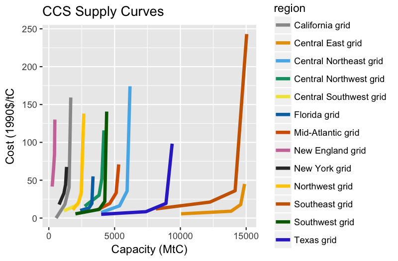
Carbon storage potential by electricity market.
Socio-economics
The socio-economic projections were developed as part of the PNNL PRIMA initiative (Scott et al. 2014). We estimate state-level medium population projections from the 2005 US Census projections from 2010 to 2030, extended to 2100 with a combination of state growth factor predictions and regression to the U.N.’s national projection. We take the ratio of the medium state projection to the national medium projection to obtain a state-to-national proportionality profile. We then apply this proportionality profile to a quantile of the national projection distribution to obtain a state’s corresponding population projection quantile (Scott et al. 2014). Historical GDP at the state level is from the Bureau of Economic Analysis (BEA, 2009). Future GDP is projected using the same aggregate productivity growth rate for all states from the GCAM Base scenario. U.S. per capita GDP in this scenario increases by 60% from 2005 to 2050 to $67,470/capita.
Referenes
Bureau of Economic Analysis, GDP by State, June 2, 2009. (http://www.bea.gov/newsreleases/regional/gdp_state/2009/gsp0609.htm)
U.S. Energy Information Agency (EIA 2008a) Annual Energy Outlook 2008 With Projections to 2030. DOE/EIA-0383(2008).
U.S. Energy Information Agency (EIA 2008b) State Energy Profile 2008 (http://www.eia.doe.gov/cneaf/electricity/st_profiles/sep2008.pdf).
U.S. Energy Information Agency (EIA 2014) State Energy Data System (www.eia.gov, downloaded 13/10/2014).
U.S. Energy Information Agency (EIA 2010) Annual Energy Outlook 2010 With Projections to 2035. DOE/EIA-0383(2010).
Scott MJ, DS Daly, Y Zhou, JS Rice, PL Patel, HC McJeon, GP Kyle, SH Kim, J Eom, and LE Clarke. 2014. “Evaluating sub-national building-energy efficiency policy options under uncertainty: Efficient sensitivity testing of alternative climate, technolgical, and socioeconomic futures in a regional intergrated-assessment model. .” Energy Economics 43(2014):22-33. doi:10.1016/j.eneco.2014.01.012
United Nations, Department of Economic and Social Affairs, Population Division (2011). World Population Prospects: The 2010 Revision, Volume I: Comprehensive Tables. ST/ESA/SER.A/313.
Zhou Y, J Eom, and LE Clarke. 2013. “The effect of climate change, population distribution, and climate mitigation on building energy use in the U.S. and China.” Climatic Change 119(3-4):979-992. doi:10.1007/s10584-013-0772-x
Calvin KV, MA Wise, GP Kyle, PL Patel, LE Clarke, and JA Edmonds. 2014. “Trade-offs of different land and bioenergy policies on the path to achieving climate targets.” Climatic Change 123(3-4):691-704. doi:10.1007/s10584-013-0897-y
Dahowski, R., Davidson, C., Dooley, J., 2011. Comparing large scale CCS deployment potential in the USA and China: A detailed analysis based on country-specific CO2 transport & storage cost curves. Energy Procedia 4, 2732-2739.
Dahowski, R., Dooley, J., Davidson, C., Bachu, S., Gupta, N., 2005. Building the Cost Curves for CO2 Storage: North America. IEA Greenhouse Gas R&D Programme, Cheltenham, UK.
Dahowski, R.T., Davidson, C.L., Li, X.C., Wei, N., 2012. A $70/tCO2 greenhouse gas mitigation backstop for China’s industrial and electric power sectors: Insights from a comprehensive CCS cost curve. International Journal of Greenhouse Gas Control 11, 73-85.
Denholm, P. and R. Margolis. 2008. Supply Curves for Rooftop Solar PV-Generated Electricity for the United States. National Renewable Energy Laboratory, Technical Report NREL / TP-6A0-44073, November 2008.
IEA. 2009. Chemical and Petrochemical Sector - Potential of best practice technology and other measures for improving energy efficiency. https://www.iea.org/publications/freepublications/publication/chemical_petrochemical_sector.pdf
Lopez A, B Roberts, D Heimiller (2012). U.S. Renewable Energy Technical Potentials: A GIS-Based Analysis. National Renewable Energy Laboratory, Technical Report NREL/TP-6A20-51946, July 2012
Luckow, P.; Wise, M.; Dooley, J. (2011_ Deployment of CCS Technologies across the Load Curve for a Competitive Electricity Market as a Function of CO2 Emissions Permit Prices, In 10th International Conference on Greenhouse Gas Control Technologies, Amsterdam, The Netherlands, 19-23 September 2010, 2011; Gale, J.; Hendriks, C.; Turkenberg, W., Eds. Elsevier: Amsterdam, The Netherlands, 2011; pp 5762-5769.
U.S. Census (2013) New Privately Owned Housing Units Completed (http://www.census.gov/construction/nrc/, downloaded 12/31/2013).
U.S. Census (2014). State Population Projections. https://www.census.gov/population/projections/data/state/
U.S. Energy Information Agency (EIA 2010) Annual Energy Outlook 2010 With Projections to 2035. DOE/EIA-0383(2010).
U.S. Energy Information Agency (EIA 2012) Table E1: Primary Energy Electricity and Total Energy Price Estimates 2012. http://www.eia.gov/state/seds/data.cfm?incfile=/state/seds/sep_sum/html/sum_pr_tot.html&sid=US
U.S. Energy Information Agency (EIA 2013a) Annual Energy Outlook 2013 With Projections to 2040. DOE/EIA-0383(2013).
U.S. Energy Information Agency (EIA 2013b) Analysis and Representation of Miscellaneous Electric Loads in NEMS. http://www.eia.gov/analysis/studies/demand/miscelectric/pdf/miscelectric.pdf
International Energy Agency (IEA 2013). Global EV Outlook: Understanding the Electric Vehicle Landscape to 2020. http://www.iea.org/publications/globalevoutlook_2013.pdf
U.S. Energy Information Agency (EIA 2014a) Annual Energy Outlook 2014 with projections to 2040 , DOE/EIA-0383(2014).
U.S. Energy Information Agency (EIA 2014b) Table 4. Biodiesel producers and production capacity by state in March 2014. http://www.eia.gov/biofuels/biodiesel/production/table4.pdf
Wise MA, JJ Dooley, P Luckow, KV Calvin, and GP Kyle. 2014. “Agriculture, Land Use, Energy and Carbon Emission Impacts of Global Biofuel Mandates to Mid-Century.” Applied Energy 114:763-773. doi:10.1016/j.apenergy.2013.08.042
Wise, M., Dooley, J., Dahowski, R., Davidson, C., 2007. Modeling the impacts of climate policy on the deployment of carbon dioxide capture and geologic storage across electric power regions in the United States. International Journal of Greenhouse Gas Control 1, 261-270.
Zhou Y, LE Clarke, J Eom, GP Kyle, PL Patel, SH Kim, JA Dirks, EA Jensen, Y Liu, JS Rice, LC Schmidt, and TE Seiple. 2014. “Modeling the effect of climate change on U.S. state-level buildings energy demands in an integrated assessment framework.” Applied Energy 113:1077-1088. doi:10.1016/j.apenergy.2013.08.034
Zhou, Y, P Luckow, SJ Smith, LE Clarke (2012) Evaluation of Global Onshore Wind Energy Potential and Generation Costs Environmental Science & Technology 46 (14) 7857-7864.