Economic Choice in GCAM

Introduction

Most of the economic activities represented in GCAM present us with a choice among several ways to produce the end result of the activity. Examples of these choices include choosing between different fuels or feed stocks, between different technologies, and between transportation modes. In some cases the choice is between different uses of a limited resource, such as when we allocate land area to different uses. In each of these cases we must allocate the total activity to the available alternatives.

Choice in GCAM is based on a single numerical value that orders the alternatives by preference. Generically, we call this the choice indicator, \(p\). In practice the choice indicator is either cost or profit rate, though other indicators are possible in principle. In cases where multiple factors influence a choice, such as passenger transportation (where faster modes are more desirable), the additional factors are converted into a cost penalty and added to the basic cost to produce a single indicator that incorporates all of the relevant factors.

Choice Functions

A function that takes as input a vector of indicators and returns a vector of market shares for the corresponding choice alternatives is called a choice function. Choice functions reflect that the single best choice does not necessarily capture the entire market. A variety of factors not captured in the model, such as individual preferences, local variations in cost, and simple happenstance cause some of the market to go to alternatives that, based on their indicator alone, are theoretically inferior choices.

GCAM provides a flexible system for specifying choice functions at runtime on a sector-by-sector basis. Choice functions are represented in the code by classes that implement the IDiscreteChoice interface. Two such classes, the Logit and the Modified Logit are currently provided.

Both of these choice functions are part of a family of that assume that the fitness of a choice alternative is a sum of two components, one determined entirely by the choice indicator (e.g., cost), and another determined by factors not captured in the model. This latter component is assumed to be random with some specified distribution. The particular distribution chosen determines the discrete choice model in use.

The Logit

The first of the two discrete choice models used by GCAM is the Logit model^[1][2]. In the Logit model the share \(s_i\) of choice alternative \(i\) (with cost \(p_i\)) is given by

\[s_i = \frac{\alpha_i \exp(\beta p_i)}{\sum_{j=1}^{N} \alpha_j \exp(\beta p_j)}.\]

In this expression, the \(\alpha_i\) are the share weights. Share weights serve two purposes in the model. First, they are used to calibrate the model to observed historical values. This calibration procedure has the effect of absorbing regionally specific preferences for particular choice alternatives (arising, for example, from societal preferences, existing infrastructure, barriers to market entry, or the like) into the share weight parameters. Share weights are also used in GCAM to provide for new technologies to be phased in gradually. GCAM accomplishes this by setting share weights for new technologies to low values in the first year they are available and gradually increasing them to a neutral value in later years.

The \(\beta\) parameter is called the logit coefficient. It determines how large a cost difference is needed to produce a given difference in market share^[3]. We can show this by writing the expression for the ratio of market shares for two options \(i\) and \(j\):

\[\frac{s_i}{s_j} = \frac{\alpha_i}{\alpha_j} \exp(\beta (p_i - p_j))\]

From this we see that the difference in market share depends (considering share weights as fixed) entirely on the cost difference, and the logit coefficient sets the scale for how large a cost difference has to be to produce a significant effect.

The Modified Logit

The second discrete choice model supported by GCAM is the Modified Logit model^[4]. In this model the share \(s_i\) is given by

\[s_i = \frac{\alpha_i p_i^\gamma}{\sum_{j=1}^{N} \alpha_j p_j^\gamma}\]

As in the Logit model, the \(\alpha_i\) are the share weights. The \(\gamma\) parameter is the logit exponent^[5]. The logit exponent performs an analogous role to the logit coefficient in the Logit model. The share ratio for this choice function is

\[\frac{s_i}{s_j} = \frac{\alpha_i}{\alpha_j} \left(\frac{p_i}{p_j}\right)^\gamma\]

Evidently, the ratio of the choice indicators serves a similar role in the Modified Logit to the difference of the indicators in the Logit. The value of the logit exponent \(\gamma\) determines how large the ratio must be to produce a significant difference in market share. One consequence of this behavior is that the Modified Logit becomes poorly behaved when one or more of the choice indicators approaches zero. GCAM handles this situation by putting a floor under the choice indicator values^[6]. Any alternative with \(p_i < 0.001\), has its share calculated as if \(p_i = 0.001\). This floor ensures that we can always calculate a valid share value, but at the cost of suppressing any response to differences in choice indicators below the floor.

Comparison of choice models

The principal difference between the Logit and Modified Logit choice models is that the former computes shares on the basis of differences in the choice indicator, while the latter uses ratios. As a result, for indicators in the typical range for GCAM, the Modified Logit is much less sensitive to incremental differences in the choice indicator^[7]. In the energy system this has the effect of allowing high-cost technologies to retain more market share than they would in the Logit case. For a gradually increasing cost adder, such as a greenhouse gas tax, it can take a long time to push uncompetitive technologies completely out of the market.

One way of understanding this behavior is by recalling that the underlying model for these discrete choice functions is of a fitness function that is partially deterministic (represented by the choice indicator, \(p\)) and partly random with a prescribed distribution. In the Logit case the distribution is the Generalized Extreme Value (GEV) distribution, while in the Modified Logit case the distribution is the Weibull distribution.

The GEV distribution The Weibull distribution
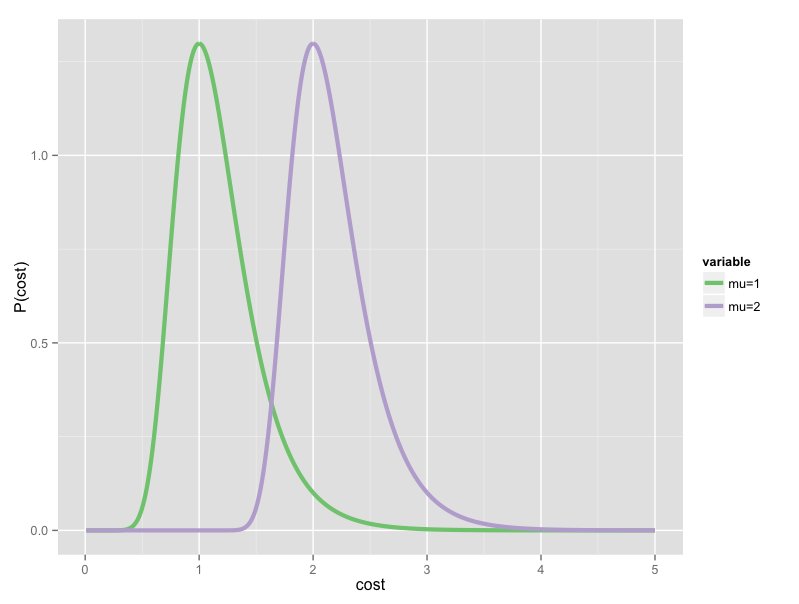
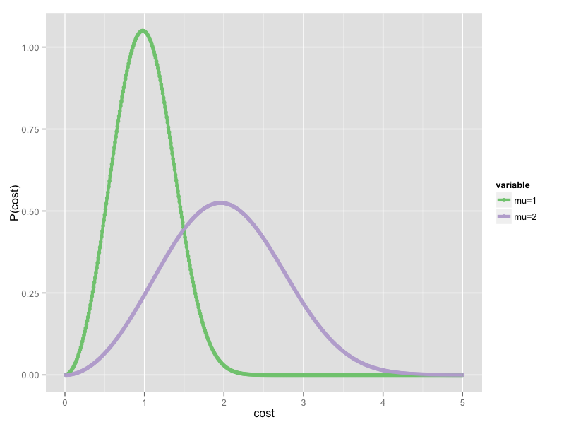
Figure 1: Comparison of the probability distributions underlying the two choice functions. Increasing the mean of the GEV (left) translates the distribution along the x-axis unchanged. Increasing the mean of the Weibull (right) also broadens the distribution.

From Figure 1 it is apparent that changing the mean of a GEV distribution while keeping its logit coefficient constant does not change the shape of the distribution. By contrast, changing the mean of a Weibull distribution while keeping the logit exponent constant makes the distribution broader or narrower. Either of these behaviors might be desirable in certain circumstances. For example, if the increase in average cost comes from applying a carbon tax, then we don’t expect the distribution of the random factors to change as a result. The Logit choice function is appropriate for this situation because its underlying GEV produces this behavior.

Conversely, in some cases a shift in cost is due to changes in secondary factors that are folded into a modified cost. For example, in passenger transportation cost is the basic contributor to the choice indicator, but people also care about the time they spend traveling. We represent this preference by adding a cost penalty to slower transportation modes. Because this penalty scales with per-capita income, it will produce a cost shift over time. In this case we would expect the distribution of the random factors in the choice model to change because the shift is a result of a change in consumer preferences, and there are many facets to consumer preference that GCAM does not capture. Therefore, in a case like this, the Modified Logit choice function is more appropriate.

GCAM Configuration

GCAM requires each sector and subsector in the energy system to have a choice function configured. Either the Logit or the Modified Logit may be selected. For historical reasons the nomenclature used in the GCAM source code and configuration files is slightly different than what is used here. The Logit and Modified Logit choice functions are referred to as “Absolute-cost Logit” and “Relative-cost Logit”, respectively. Additionally, the logit coefficient for the Logit model is not specified directly. Instead, a logit exponent for an equivalent^[8] Modified Logit model is specified, and GCAM calculates the corresponding logit coefficient. This allows users to switch easily from Logit to Modified Logit or vice versa without recalculating the parameters.

A choice function is specified by including its declaration in the sector to which it will pertain. Consider this excerpt from the GCAM Reference Scenario (GRS) configuration:

         <supplysector name="electricity">
            <relative-cost-logit>
               <logit-exponent fillout="1" year="1975">-3</logit-exponent>
            </relative-cost-logit>

   . . .

            <subsector name="coal">
               <relative-cost-logit>
                  <logit-exponent fillout="1" year="1975">-10</logit-exponent>
               </relative-cost-logit>
			   
   . . . 

This snippet configures the Electricity sector with a Modified Logit choice function for allocating market shares to the available subsectors. (Each subsector represents a different fuel input.) The logit exponent for this choice function is -3, which turns out to provide moderate switching behavior when costs change. Further down we configure the Coal subsector with a Modified Logit for allocating shares to its subsidiary technologies. (These represent different plant designs, such as steam or IGCC.) The logit exponent in this case is -10, which produces more aggressive switching behavior with changing costs.

Either of these declarations could be changed to the Logit choice function by changing the <relative-cost-logit> XML tag to <absolute-cost-logit>. The <logit-exponent> tag could be left alone to produce a choice function that is similar to the Modified Logit version for costs close to those found in the calibration year. However, the behaviors of the two functions will diverge as costs move out of this initial range.

The choice model in the land system is not currently configurable like in the energy system. Instead, land use choices are always made using the Modified Logit. Logit exponents are specified directly in the container object using the <logit-exponent> tag. Land use choice is described further in the Agriculture and Land Use chapter.

Notes and References

[1] Train, K. (2003), Discrete Choice Methods with Simulation.

[2] McFadden, D. (1973), “Conditional Logit Analysis of Qualitative Choice Behavior”, in Frontiers in Econometrics.

[3] The logit coefficient \(\beta\) may be either positive or negative, depending on the interpretation of the choice indicator \(p\). Having \(\beta < 0\) favors lower values of \(p\) and is therefore appropriate when \(p\) represents cost (the usual case in GCAM). In the land system the choice indicator represents profit rate, and we use \(\beta > 0\) in these choice functions to favor higher profit rates.

[4] Clarke, J. F. and Edmonds, J. (1993), “Modeling energy technologies in a competitive market”, Energy Economics 15 (2), 123 - 129.

[5] As with the \(\beta\) coefficient in the Logit model, the sign of \(\gamma\) depends on the interpretation of the choice indicator, with negative values favoring smaller \(p\) and positive values favoring larger \(p\).

[6] This statement is actually only true in the energy system. In the land system (where the choice indicator is the profit rate), shares are calculated normally for all \(p>0\). For \(p\leq0\) the share is automatically set to zero.

[7] This is not universally true. For \(p \ll 1\) tiny increments in \(p\) can produce huge share differences. For most of GCAM, where \(p\) represents cost, values in this range are uncommon, but they do occur in a few sectors.

[8] By suitable choice of parameters, one can arrange for the Logit and Modified Logit to have similar behavior in some neighborhood of input values. However, this equivalence is approximate, and the two choice functions diverge increasingly, the further the inputs get from this neighborhood of equivalence. Typically we choose this neighborhood to be the costs during the calibration period, but if necessary it can be specified explicitly with the <base-cost> XML tag inside the choice function declaration.