Agriculture, Land-Use, and Bioenergy

In GCAM, the model data for the agriculture and land use parts of the model comprises 283 subregions in terms of land use, based on a division of the extant agro-ecological zones (AEZs), which we derived from work performed for the GTAP project (Monfreda et al, 2009), within each of GCAM’s 32 global geo-political regions. Within each of these 283 subregions, land is categorized into approximately a dozen types based on cover and use. Some of these types, such as tundra and desert, are not considered arable. Among arable land types, further divisions are made for lands historically in non-commercial uses such as forests and grasslands as well as commercial forestlands and croplands. Production of approximately twenty crops is currently modeled, with yields of each specific to each of the 283 subregions. The model is designed to allow specification of different options for future crop management for each crop in each subregion.

AgLU Inputs and Outputs

This section briefly summarizes inputs and outputs, including data sources, spatial and temporal resolution. A more complete description of data is available in PNNL Technical Report 21025.

Inputs

GCAM’s inputs include information on production, consumption, prices, land, carbon, and other emissions in the historical period. GCAM requires globally consistent data sets for each of its historical model periods. The GCAM data system can produce such data sets annually beginning in 1971. Currently, GCAM uses data from 1990, 2005, and 2010 to initialize the model, but could be initialized to any year beginning in 1971.

Production: Inputs include production of all crops and forestry products for each of the 283 AgLU regions. We currently rely on a blend of FAO and GTAP data for these inputs. FAO includes country-level data over the entire historical period, while GCAM has sub-national information for a single year in time.
Consumption: Inputs include food, non-food, bioenergy, and feed consumption of all crop and forestry products for each of the 32 geopolitical regions. We currently rely on IMAGE for animal feed and FAO data for all remaining inputs.
Prices: Inputs include the price of all food, feed, and forestry commodities. We currently use producer prices from FAO for these inputs.
Land: Inputs include land cover and land use for each of the GCAM land types and AgLU regions. We use information beginning in 1700 in order to spin-up the carbon cycle within GCAM. Currently, we use a blend of the Hurtt-Hyde land cover product from CMIP5, the SAGE potential vegetation map, and FAO/GTAP cropland area.
Carbon: Inputs include potential vegetation and soil carbon density (i.e., carbon density if the land grew to equilibrium) and a mature age. Currently, we derive vegetation carbon densities for crops from the FAO computed crop yield. All other carbon densities and mature ages come from Houghton (1999) and King (1997).
Other Emissions: Inputs include emissions of all non-CO₂ gases and species for each year and region. Data for BC and OC is from the RCP inventory (Lamarque et al., 2011). Data for all other gases and species is from EDGAR (European Commission, 2010).

Outputs

GCAM’s outputs include variables related to production, consumption, prices, land, carbon, and other emissions.

Production: Outputs include production of all crops and forestry products; this information is calculated annually for each of the 283 AgLU regions. GCAM also calculates production of livestock at the 32 region level.
Consumption: Outputs include food, non-food, bioenergy, and feed consumption of all crop, forestry, livestock, and bioenergy products; this information is calculated annually for each of the 32 geopolitical regions.
Prices: Outputs include the price of all food, feed, forestry, bioenergy and livestock commodities. This information is calculated annually, typically at a global level; however, some commodities (e.g., livestock) have regional prices (32-region level).
Land: Outputs include land use and land cover for each of the land types included in GCAM (see Figure 1). This information is calculated annually for each of the 283 AgLU regions.
Carbon: Outputs include carbon stock and land-use change emissions of CO₂. This information is calculated annually for each of the 283 AgLU regions.
Other emissions: Outputs include emissions of CH₄, N₂O, NH₃, SO₂, CO, BC, OC, and NO_x. Greenhouse gas emissions are produced from livestock, rice, and fertilizer application; these emissions can be reduced with the application of a carbon price. Pollutant emissions are produced from agricultural waste burning, forest fires, deforestation, and savannah burning. Livestock emissions are calculated annually at the 32 region level. All other emissions are calculated annually at the 283 region level.

Economic Modeling Approach

In this section, we describe and discuss the approach we have developed for the economic modeling of agriculture, forestry, and land use in the Global Change Assessment Model (GCAM). We discuss the math determining land allocation in the model, as well as its interpretation. We explain the land nesting strategy and its implications, the math used in calibrating the model, and the types of data required for calibration (the data itself is discussed in later sections). We finish this section with an explanation and discussion of methods for introducing new crops and technologies into the competition beyond the calibration year. More information, including a comparison to other models, is available in Wise et al. (2014).

Economic land use decisions in GCAM are based on a logit model of sharing based on relative inherent profitability of using land for competing purposes. The logit approach was developed by McFadden (1974) to describe the distribution of consumer choice, but a similar mathematical approach works well here for our purposes. The interpretation of this sharing system in GCAM is that there is a distribution of profit behind each competing land use within a region, rather than a single point value. Each competing land use option has a potential average profit over its entire distribution. The share of land allocated to any given use is based on the probability that that use has a highest profit among the competing uses. The relative potential average profits are used in the logit formulation, where an option with a higher average profit will get a higher share than one with a lower average profit. However, at the margin, the profits of competing options are equal. In essence, the sharing can therefore be considered optimal, but the assumption of a distribution of profits makes it very different from a constrained linear optimization approach.

In GCAM, competing uses of land are nested within land nodes. Within each land node, it is generally assumed to be easier to substitute products, so logit exponents are higher to indicate tighter competition. Examples include switching food crops from one to another and converting forests from unmanaged categories to logging forests. Substitution across land nodes is also allowed but is assumed to be more difficult than within land nodes. We implement this philosophy by setting lower logit exponents via input data. For example, the expansion of cropland into pasture is more difficult than expansion of wheat land into corn land.

Although relative average profit rates are used in the logit sharing equations, the theory behind the math is that land shares are determined so the land is allocated across uses up until the point at which the marginal profit rates are equal to each other. Therefore, the land values at the margin are also equal. As a result, all land uses within a nesting structure have equal value at the margin and further substitution will not increase total profits. If one option has a higher potential average profit rate than a second, it is assumed that option has a greater proportion of its distribution of profit rates that will exceed the marginal profit rate than the second option. Therefore, this option will receive a higher share, but unlike a simple optimization model it will not get all of the land in the node.

Land Nesting Strategy

The strategy for nesting competing land uses and nesting nests of competing land uses has involved some expert judgment, as does the choice of logit exponents that govern substitution within each of the level of the nesting structure. Note that calibration and reproduction of historical results does not depend on the nesting strategy or the logit exponents used. Instead, these assumptions affect future period results as conditions or policies change from history.

Before discussing our nesting approach, it is useful to consider the space of possible nesting strategies. One approach is that of a single nest: the assumption that the land regions are small enough that all competing options are equally substitutable. This assumption implies that it is just as easy to switch from forest to wheat as it is to switch from corn to wheat. However, this conversion would not happen unless wheat was more profitable than forest or corn. With a high enough logit exponent for this single nest, the land sharing approaches an optimal “winner-take-all” result in that all land within a region will be dedicated to the most profitable product in that region. A single nest with a high exponent represents the extreme end of unconstrained optimization in which there is no transition cost or other hurdle for switching from one land type to another.

The other extreme is that of no substitution. This would be accomplished with near zero or zero logit exponents, whether in a single nest or multiple nests. This implies that either it is physically impossible or the transition costs are too high to allow switching from one land type to another. Currently, in GCAM, we use zero logit exponents in a very limited number of situations, where we do not want any substitution (e.g., we do not allow cropland to expand into desert or tundra). However, in most situations, we employ positive logit exponents and allow economics to dictate the land allocation within a region.

Our approach is to use a nesting strategy that allows the logit exponents to reflect differences in substitutability across land categories. Figure 1 shows the nesting diagram of land with an AEZ subregion. At the top is all land, which is divided into two main types of nodes: agro-forestry land and the remaining categories of land that are not suitable for agriculture. This second category could be divided further if useful. The next node layer contains two further nodes: all agro-forestry, non-pasture land and all pasture land. The pasture land node contains two competing uses (land leaves in the code): managed pasture (that which feeds marketed livestock) and unmanaged pasture.

AgLU Land Nesting Diagram
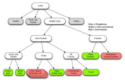
Figure 1: AgLU Land Nest

The agro-forestry (non-pasture) node contains three competing nodes: shrub and grass lands, forest lands, and croplands. Shrublands and grasslands are separated from the rest as they are both classified as unmanaged land categories and we want to control their substitutability between each other separately. Finally, the forestland node competes with the total cropland node. Within forestland, there are managed and unmanaged forest leaves, and we have added a woody biomass option there in some regions and scenarios. Under cropland are all food and other agriculture products (e.g., corn, wheat, sugars, etc.), including biomass crops, along with an unmanaged land category called other arable land. Note that several crops are included explicitly in the CropLand node, and the grouping of “AllOtherCrops” is simply a convenience for this figure.

With this specification, we can make substitution across categories more or less difficult by choosing lower or higher logit parameters.

Calibration

While the profit-based logit land sharing is fairly straightforward, it must be calibrated to match historical data on land use shares, crop yields, costs, and land prices in the base year. The calibration method is algebraically simple, but it can be difficult conceptually. The aim of the calibration is to infer distributions and underlying parameters from the historical data. Based on the logit model chosen, including nesting and exponents, underlying economic values of the various land types are implied from the real world shares of each land.

For calibration, base year data sets must include values of physical results such as land use, agriculture and forest production, demand for all agricultural and forestry products, product yields per unit of land, and other data such as carbon densities. The calibration data also needs to include product prices and land prices.

The approach to calibration is to solve for parameters that adjust observed profit rates, which are based on base year data, such that they equal the potential average profit rates implied by base year shares and the assumed average price of unmanaged land. The potential average profit rates implied by the shares can be interpreted as the average profit if all land were devoted to that use. Here, we will refer to these rates as the calibration profit rates. The calibration parameters, which we have called calibration profit scalers in the code, should not be confused with the logit share weights that we use in the energy model. They serve much the same function, but their derivation is more complicated, and they should not be assumed to be transformable. Unlike the share weights, the absolute values of the calibration profit scalers have meaning, not just their relative values. Therefore, they cannot be transformed by indexing them around a value of one for convenience like we can do with the share weights in the energy sector.

In future model periods, the calibration profit scalers are used to adjust the future profit rates in the logit sharing and profit equations. The calibration routine ensures that the future is grounded in history. If prices, demand, and crop yields were unchanged in future modeling periods, shares, profits, and land allocations would equal the base year values. When future conditions evolve in the model such that costs, prices, yields, and other factors deviate from historical values, shares and profits will also change from their base year values.

Variable Costs

Variable costs are defined here as the non-land costs of crop production, per-unit of crop. Variable costs set hard price floors in the model: production goes to zero when price is less than or equal to the variable costs. As a result, these costs should be interpreted as pure minimum or shut-down costs. They should be just the cost of materials and hired labor for producing a crop or product with a given technology in a subregion.

Value-added categories should not be included in the variable costs. In addition, variable costs should not include land costs, as the model is based on allocating land on per unit profits. They should also not include cost categories that represent return to capital or profits. We can assume these costs are captured in the distribution of profit rates behind the logit. Otherwise, consider that if these costs are put into our variable costs, ultimately all marginal profit rates (from economic theory) would be zero and provide no value to our modeling. In addition, accounting costs such as depreciation should not be part of variable costs.

Data on labor costs can be difficult to use, since some farm wage categories are income that the farmer either earns or expects to be paid and thus, some labor costs are really profit to the land-owner (i.e., farmer). Therefore, we have restricted our variable cost data to include what is labeled as “hired labor”.

Note that introducing variable costs that differ by region can result in unintended consequences. Different variable costs create different price floors, which can result in a region ceasing production of a particular product if technical change lowers the global product price significantly (i.e., to a point where the variable cost is less than the price received).

The main points can be summarized as:

Variable costs create price floors
Variable costs should be based on technology data. They should not be used as calibration parameters to adjust profits.
Variable costs should not include value-added categories of land, return to capital, and owner-wages.

New Land Types

The calibration process can accommodate gaps or imprecisions of the price and cost data for the crops and land uses in base year calibration data set. Changing the values of inputs such as land prices, product prices, and product variable costs will change the values of the calibration parameters internal to the model. Algebraically, the calibration parameters adjust or compensate to make the profit rates consistent with the base year shares and crop yields. In most situations, these changes will not affect model results either in the calibration year or future years. The calibration is to an extent self-correcting.

However, there are a few important exceptions to this rule. First, as previously noted, variable costs introduce price floors and thus, increasing these values may result in some regions ceasing production in future years. Second, exceptions occur when we introduce crops, technologies, or policies that are not part of the base year calibration data set. One example is when new biomass crops are introduced. To introduce a new crop or a new crop technology, the model has to evaluate how its profitability compares to all other crops and uses of land. In this case, the actual values of the prices and costs that determine profits do matter. In the biomass example, it is important not only to have the variable costs and yields of the biomass correct, we also have to have the magnitudes of the profits of the competing crops correct for the competition to be valid. That means we have to have the prices and costs for all of the crops correct. Calibration cannot compensate for this problem.

The same would be true for introducing new technologies for growing existing crops that are part of the calibration data set. For example, if we introduce a new management technique for growing corn to compete with the existing technique, the variable costs for both the new technology and the existing technology would have to be correct for the competition to be valid.

Land prices are for the most part factored out by the calibration. They behave almost like numeraires, with at least one important exception. Land prices, along with land shares, set the values for unmanaged land categories. At the margin, we assume the value of unmanaged land is equal to the land price. This is of course also true of managed land categories, but unmanaged lands are special in that they do not produce a product other than this intrinsic value represented by the land price. The land price becomes important when we introduce a carbon subsidy on land, as the amount of the subsidy relative to the land price will determine its impact. For example, if the land price is high, a carbon subsidy may have a small impact on the relative value of unmanaged land. However, if the land price is low, the same carbon subsidy will have a higher relative impact on the value of unmanaged land. We see this effect in the model where there is a greater response to a carbon subsidy in regions with lower land prices.

Crop Outliers: The Special but Common Case of a High-Yielding Crop in a Very Small Section of a Region

There are many places in the crop production data where a small amount of land produces a crop at a high yield that is not representative of the potential yield of that region. Some of these cases are data errors, but some cases are real observations where crop production is intensively managed or irrigated. In the current calibration data set, the amount of food, fiber, and fodder produced in these high-yielding regions is small relative to regional or global crop production. Through the calibration process, we have ensured that the model cannot expand that these high-yielding crops throughout that region without substantial costs.

For example, the current data set has very high-yielding wheat in the panhandle of Alaska. The data suggest that there is a very small amount of land producing wheat with a very high yield. This wheat land accounts for a small share of cropland in that AEZ. Because the share of cropland is low, the calibration process will compute parameters that reflect limitations on the potential expansion of this land due to cost or factors not otherwise modeled. Literally, the math will calculate very low profit share scalers for wheat in Alaska. This also is the case if wheat share of cropland is high but the cropland share of arable land is low, implying something is preventing cropland from expanding. Perhaps the real world cropland extent reflects something about the soil quality that is not explicitly modeled in AgLU.

Regional Production and Comparative Advantage

In its determination of the economic allocation of crop production and land use across regions of the globe, GCAM follows the well-known but often misunderstood basic economic principle of comparative advantage. The theory of comparative advantage was identified and explained by David Ricardo in the early 19th Century (Ricardo, 1817) to explain patterns in the study of international production and trade (Samuelson and Nordhaus, 2004). In simplest terms, countries or regions will produce more of what they are better at and import more of what they are not as good at producing.

This appears obvious, but the distinction between comparative advantage and an “absolute” advantage is often confused. First, consider a situation of two crop products, Crop 1 and Crop 2 produced in two countries, A and B. The solution is trivial if Country A produces Crop 1 better (at a higher profit) than Country B while Country B produces Crop 2 better than Country A. In this example, Country A will tend to produce more of Crop 1 to export to Country B while importing more of Crop 2 from Country B, and the world is better off from the trade. Although the principle of comparative advantage is satisfied here, the fact that it also a situation of absolute advantage trivializes the concept and is not fully explanatory.

To clarify the distinction between absolute and comparative advantage, consider a more realistic situation in which Region A has higher yields and lower costs of producing both Crop 1 and Crop 2 than Region B: Region A has an absolute advantage over Region B in both crops. Does that mean Region A will grow both crops and Region B will grow nothing? Clearly not. Assume that Crop 1 has a much higher value or price than Crop 2. The comparative advantage solution is that will be that Region A will maximize it profits by growing more of Crop 1 and exporting it to Region B. This will leave a market opportunity for Region B to specialize in Crop 2 and export it to Region A. Region B has a comparative advantage in Crop 2 and thus have higher profits than if it grew Crop 1, for which it would not be competitive with Region A.

The GCAM representation of global land and allocation is much more complicated than this simple example in modeling economic decisions as it assumes a distribution of profit rates over land areas and must be calibrated to reflect real-world data where regions grow a mix of crops rather than completely specializing. However, the simple example above is relevant and powerful in interpreting GCAM’s approach and results. Within each land use subregion in GCAM, economic uses of land are allocated based on that subregion’s own relative profit rate distributions of agriculture, forestry, and other competing uses for land. In essence, this means that land use allocations are based on comparative advantage rather than absolute advantage. Within a land subregion, land use allocations are based on what it can earn the higher profit rates among its own set of options, not what its yields or its profit rates are compared with the rest of the globe. That is, a farmer in an individual region will choose to grow the crop that results in the highest profit, regardless of how his profit/yield for that crop compares to the profit/yield of that crop in other regions.

Consider the example of a future scenario with a high global demand for a bioenergy crop such as switchgrass. A developed region with favorable climate such as Western Europe may have much higher potential yields, and thus higher potential profit rates for growing a bioenergy crop than Africa. However, that does not mean that Western Europe would grow more bioenergy crops than Africa. Western Europe will also have higher yields and profits for high-valued food crops, as well as high land prices that would limit expansion of agricultural land. Africa may find in this scenario that it is profitable to expand agricultural land for bioenergy crops for export, even though its bioenergy yields are lower on an absolute basis. Similar examples can be made with food crops and forestry.

Although GCAM is not structured as an optimization model, the allocation of production of crops and products across regions and subregions of the globe based on comparative advantage can be considered optimal in terms of maximizing global profits (which is not the same as minimizing land requirements). While each land subregion makes its own independent allocation, the subregions communicate these decisions with each other through economic markets. The global markets for agricultural and forest products react to these allocations by comparing global supplies to demands and adjusting prices to equilibrate supplies and demands. The resulting prices are sent back to each land subregion as signals as to how its land allocation should be changed. The process of allocation and price adjustment continues until the markets are in equilibrium. This market equilibrium is an economically efficient allocation of land resources among regions (Samuelson and Nordhaus, 1985).

Terrestrial Carbon Approach

Land-use change CO₂ emissions are calculated in GCAM using a simple accounting approach, similar to that of Houghton (1999). That is, GCAM determines the change in above and below ground carbon stock for a given land use change and allocates that change in carbon stock over time.

Vegetation Carbon

For vegetation carbon, we distinguish between two different activities – land expansion and land contraction. In the event that land contracts, i.e., there is less land in the current period than the previous period, we assume that all emissions are released instantaneously. In this event, the land-use change emissions for the current period from above ground carbon changes are equal to the change in above ground carbon stock. Emissions from above ground carbon changes for all other periods are equal to zero. In the event land expands, we spread the change in carbon stock across time depending on the length of time it takes for the vegetation to mature. For crops, the mature age is typically set a 1 year, meaning that all carbon uptake occurs instantaneously. For forests, however, we assume it takes anywhere from 30 years to 100 years to uptake all of the carbon. We use an example of the Bertalanffy-Richards function.

Soil Carbon

For soil carbon, we assume we assume both emissions and uptake are exponential, where the exponential half-life depends on the region. Colder regions have longer half-lives.

Carbon Stocks

GCAM tracks carbon stocks by calculating and storing cumulative land-use change emissions, and then applying those emissions as time proceeds. As land expands, we compute future uptake to be added to the carbon stock, and as land contracts we compute future emissions to subtract from the carbon stock.

Policy Options

This section summarized some of the land-based policy options available in GCAM. More information on the trade-offs of these options is available in Calvin et al. (2014).

Protecting Lands

With this policy, we can set aside some land, removing it from economic competition. This will result in that land area being fixed across time and any land expansion/contraction will not affect this area. The default in GCAM is to protect 90% of all non-commercial ecosystems.

Valuing Carbon in Land

In a policy regime, we can choose to put a price on land-use change CO₂ emissions that is related to the price on fossil fuel and industrial CO₂ emissions. The land carbon price can be any multiplier of the fossil fuel carbon price. This factor is applied at the geopolitical region level, and can be differentiated across regions. We model this policy as a subsidy to land-owners for the holding carbon stocks, as opposed to a tax/subsidy on the change in carbon in land. Specifically, the subsidy is equal to the carbon price x the carbon density x a discount factor to account for the amount of time it takes carbon to accumulate x a discount factor to annualize the subsidy.

Bioenergy Constraints

We can impose constraints (lower or upper bounds) on bioenergy within GCAM. Under such a policy, GCAM will calculate the tax or subsidy required to ensure that the constraint is met.

Land expansion costs/constraints

One approach we have implemented and tested is to add a land expansion cost curve to targeted land types in regional AEZs. Specifically, we have added land expansion cost curves to unmanaged forest land in regional AEZ’s in which a carbon policy resulted in fast transformation from grassland to unmanaged forest. This method effectively adds a cost associated with converting to forests. This cost can be interpreted as the cost of planting, watering, fire management, etc. required to grow trees on previously unforested land.

The land expansion cost curve is implemented as a “renewable” resource that land must “purchase” on a per-unit of land basis. The cost curve can be set at a zero cost up to a predefined amount of land: e.g., base year allocation, pre-industrial allocation, etc. Beyond this point, the cost curve increases to either represent a physical expansion cost or an arbitrarily high cost that would act as a hard constraint on expansion. One drawback to this approach is that each cost curve adds a market equation that needs to be solved. The market should behave well, but adding markets should always be done with care as it does put additional burdens on the solution algorithm.

Carbon Parks

We have also included code to implement a crop technology that plants trees as densely as possible just for the purposes of storing carbon. Such a “carbon park” technology would allow us to explicitly include physical costs and demands for other inputs such as fertilizer and water when that modeling is available. This would clearly be a “managed” land option and would allow us some more options for modeling carbon policies. As with expansion costs/constraints, carbon parks are not a part of the current core configuration, but can be implemented through changes in input files.

References

Beach, Robert and Bruce McCarl. 2010. US Agricultural and Forestry Impacts of the Energy Independence and Security Act: FASOM Results and Model Description. RTI International. Research Triangle Park, NC.

Birur, Dileep K., Thomas W. Hertel, and Wallace E. Tyner, 2008. Impact Of Biofuel Production On World Agricultural Markets: A Computable General Equilibrium Analysis. GTAP Technical Paper No. 53. https://www.gtap.agecon.purdue.edu.

Brenkert A, S Smith, S Kim, and H Pitcher. 2003. Model Documentation for the MiniCAM. PNNL-14337, Pacific Northwest National Laboratory, Richland, Washington. Available at: http://www.globalchange.umd.edu/models/MiniCAM.pdf

Burniaux, Jean-Marc and Truong P. Truong, 2002. GTAP-E: An Energy-Environmental Version of the GTAP Model. GTAP Technical Paper No. 16. https://www.gtap.agecon.purdue.edu.

CARD Staff, 2009. An Analysis of EPA Renewable Fuel Scenarios with the FAPRI-CARD International Models. Technical Report. 2009.

Calvin, K., M. Wise, P. Kyle, P. Patel, L. Clarke and J. Edmonds (2014). “Trade-offs of different land and bioenergy policies on the path to achieving climate targets.” Climatic Change 123(3-4): 691-704.

Clarke, J.F. and Edmonds, J.A. (1993) ‘Modelling Energy Technologies in a Competitive Market’, Energy Economics, 15: 123-129.

Clarke, L., J. Lurz, M. Wise, J. Edmonds, S. Kim, S. Smith, H. Pitcher. 2007. Model Documentation for the MiniCAM Climate Change Science Program Stabilization Scenarios: CCSP Product 2.1a. PNNL Technical Report. PNNL-16735.

Edmonds, J. and J. Reilly. 1983. “Global Energy Production and Use to the Year 2050,” Energy, 8(6):419-32

Edmonds, J. and J. Reilly. 1983. “Global Energy and CO2 to the Year 2050,” The Energy Journal, 4(3):21-47.

Edmonds, J. and J. Reilly. 1983. “A Long-Term, Global, Energy-Economic Model of Carbon Dioxide Release From Fossil Fuel Use,” Energy Economics, 5(2):74-88.

Edmonds, J.A., Reilly, J.M., Gardner, R.H., and Brenkert, A. 1986. Uncertainty in Future Global Energy Use and Fossil Fuel CO2 Emissions 1975 to 2075, TR036, DOE/NBB-0081 Dist. Category UC-11, National Technical Information Service, U.S. Department of Commerce, Springfield Virginia 22161.

European Commission, Joint Research Centre (JRC)/PBL Netherlands Environmental Assessment Agency. Emission Database for Global Atmospheric Research (EDGAR), release version 4.2. http://edgar.jrc.ec.europe.eu, 2010

FAPRI, 2011. FAPRI Models. http://www.fapri.iastate.edu/models/. Retrieved November 8, 2011.

GTAP, 2011. About GTAP: Center for Global Trade Analysis. https://www.gtap.agecon.purdue.edu/about/center.asp. Retrieved November 9, 2011.

Gurgel, A., J. Reilly, S. Paltsev (2007). “Potential Land Use Implications of a Global Biofuels Industry.” Journal of Agricultural and Food Industrial Organization 5(2), 1202.

Hartin, C. A., Patel, P., Schwarber, A., Link, R. P., and Bond-Lamberty, B. P.: A simple object-oriented and open-source model for scientific and policy analyses of the global climate system – Hector v1.0, Geosci. Model Dev., 8, 939-955, doi:10.5194/gmd-8-939-2015, 2015.

Havlík, P., Schneider, A.U., Schmid, E., Böttcher, H., Fritz, S., Skalský, R., Aoki, K., de Cara, S., Kindermann, G., Kraxner, F., Leduc, S., McCallum, I., Mosnier, A, Sauer, T. and Obersteiner, M. (2011). Global land-use implications of first and second generation biofuel targets. Energy Policy 39: 5690-5702.

Houghton, R.A. 1999. The annual net flux of carbon to the atmosphere from changes in land use 1850-1990. Tellus 51B: 298-313.

King, A. W., Post, W. M., and Wullschleger, S. D. 1997. The potential response of terrestrial carbon storage to changes in climate and atmospheric CO2. Climatic Change, 35(2), 199–227. Springer. Retrieved March 9, 2011, from http://www.springerlink.com/index/K528446L38325833.pdf.

Lamarque, J.-F., G. P. Kyle, M. Meinshausen, K. Riahi, S. Smith, D. van Vuuren, A. Conley and F. Vitt (2011). “Global and regional evolution of short-lived radiatively-active gases and aerosols in the Representative Concentration Pathways.” Climatic Change 109(1-2): 191-212.

Monfreda, C., N. Ramankutty and T. W. Hertel (2007). Global Agricultural Land Use Data for Climate Change Analysis. in Economic Analysis of Land Use in Global Climate Change Policy. T. W. Hertel, S. Rose and R. S. J. Tol, Routledge.

Raper, S. C. B. and U. Cubasch (1996) Emulation of the results from a coupled general circulation model using a simple climate model GEOPHYSICAL RESEARCH LETTERS, VOL. 23, NO. 10, PP. 1107-1110 doi:10.1029/96GL01065

Ricardo, D. (1817). On the Principles of Political Economy and Taxation, London.

Samuelson, Paul A.; William D Nordhaus (2004), Economics, McGraw-Hill, ISBN 0-07-287205-5

Sands, R.D. and Leimbach, M. (2003) ‘Modeling Agriculture and Land Use in an Integrated Assessment Framework’, Climatic Change, 56: 185-210.

Taheripour, Farzad, Wallace E. Tyner and Michael Q. Wang, 2011. Global Land Use Changes due to the U.S. Cellulosic Biofuel Program Simulated with the GTAP Model. https://www.gtap.agecon.purdue.edu.

U.S. Department of Energy. 2011. U.S. Billion-Ton Update: Biomass Supply for a Bioenergy and Bioproducts Industry. R.D. Perlack and B.J Stokes (Leads), ORNL/TM-2011/224. Oak Ridge National Laboratory, Oak Ridge, TN. http://bioenergykdf.net.

University of Tennessee. 2011. The Polysys Modeling Framework: a Documentation. Agriculture Policy Analysis Center. http://www.agpolicy.org/polysys.html. Retrieved September 10, 2011.

Wigley, T. and S. Raper (1992). “Implications for Climate and Sea-Level of Revised IPCC Emissions Scenarios.” Nature 357(6376): 293-300.

Wigley, T.M.L. and Raper, S.C.B. 2002. Reasons for larger warming projections in the IPCC Third Assessment Report J. Climate 15, 2945–2952.

Wise, M., K. Calvin, A. Thomson, L. Clarke, B. Bond-Lamberty, R. Sands, S. J. Smith, A. Janetos and J. Edmonds (2009). “Implications of Limiting CO2 Concentrations for Land Use and Energy.” Science, Volume 324(5931): 1183-1186 DOI:10.1126/science.1168475

Wise, Marshall, Calvin, Katherine, Page Kyle, Patrick Luckow, James Edmonds. 2014. Economic and Physical Modeling of Land Use in GCAM 3.0 and an Application to Agricultural Productivity, Land, and Terrestrial Carbon. Climate Change Economics. DOI 10.1142/S2010007814500031.